[PoreSpy]提取纤维孔隙网络模型过程验证
1.验证过程
1.1 导入纤维CT图像
import imageio.v2 as imageio
import porespy as ps
import numpy as np
from matplotlib.pyplot import subplots
import scipy.ndimage as spim
from skimage.restoration import non_local_means, estimate_sigma
from skimage.io import imread_collection_wrapper,imread,imread_collection
import matplotlib.pyplot as plt
import time
import os
from skimage import io

#imageio包里内置读取3D图像的函数imageio.volread
im=imageio.volread('C:\\Users\\ALPHA\\Desktop\\PNM\\object\\test3-3D.tif')
fig, ax = plt.subplots()
ax.imshow(ps.visualization.show_planes(im), cmap='gray');#显示3D图像的三视图,以灰度图的方式打开
def volread(uri, format=None, **kwargs):
    """volread(uri, format=None, **kwargs)

    Reads a volume from the specified file. Returns a numpy array, which
    comes with a dict of meta data at its 'meta' attribute.

    Parameters
    ----------
    uri : {str, pathlib.Path, bytes, file}
        The resource to load the volume from, e.g. a filename, pathlib.Path,
        http address or file object, see the docs for more info.
    format : str
        The format to use to read the file. By default imageio selects
        the appropriate for you based on the filename and its contents.
    kwargs : ...
        Further keyword arguments are passed to the reader. See :func:`.help`
        to see what arguments are available for a particular format.
    """
Micro-CT的图片可以是3D模型也可以是一个包含所有切片图像的文件,这里我先将切片文件夹整合成3D图片tif格式,方法参考:
[PoreSpy] 图像导入和基本处理
生成的灰度三视图如下
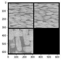
从图中可以看出纤维形态边界比较模糊,这是因为存在噪声,下面采用skimage包里的过滤器函数进行消噪
1.2 消噪
在上个笔记中我们详细观察了几种过滤函数的效果
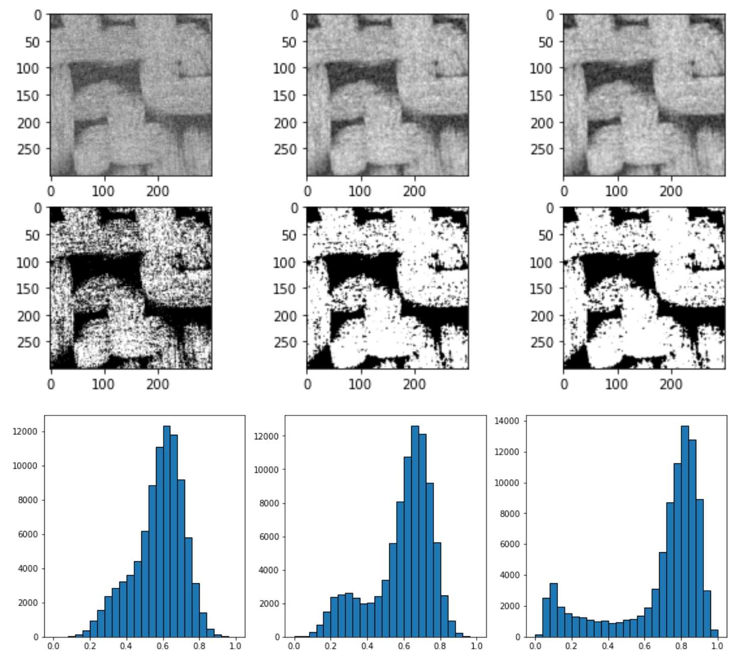
上图中从左到右依次是直接平均灰度值im = (im - im.min())/(im.max() - im.min()),均质过滤spim.uniform_filter(im, size=3),高斯过滤spim.gaussian_filter(im, sigma=1)
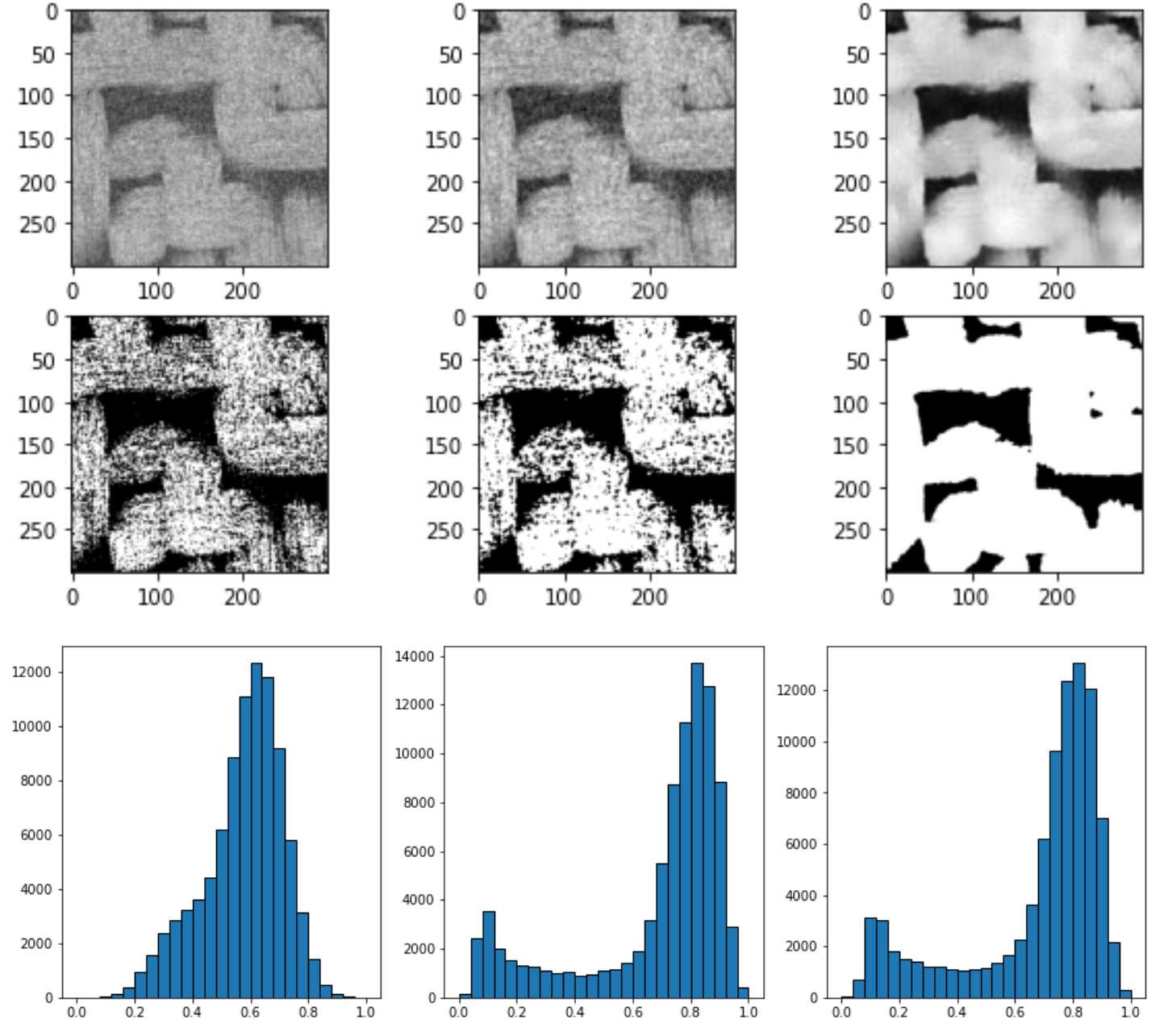
上图中从左到右依次是直接平均灰度值,中值过滤spim.median_filter(im, size=3),非局部均值过滤skimage.restoration.non_local_means.denoise_nl_means
可以看到非均值过滤器的过滤效果最好,灰度分布图可以看到图像被分为两个部分及明相和暗相,因此直接采用非局部均值过滤器skimage.restoration.non_local_means.denoise_nl_means进行噪声过滤
im = (im - im.min())/(im.max() - im.min())#对原图灰度值直接平均
s = estimate_sigma(im)

start =time.time()
im1 = non_local_means.denoise_nl_means(im)
im1 = (im1 - im1.min())/(im1.max() - im1.min())
end = time.time()
print('Running time: %s Seconds'%(end-start))
fig, ax = plt.subplots()
ax.imshow(ps.visualization.show_planes(im1<0.4), cmap='gray');
fig, ax = subplots(1, 2, figsize=[10, 5])
ax[0].hist(im.flatten(), bins=25, edgecolor='k')
ax[1].hist(im1.flatten(), bins=25, edgecolor='k')
'''
Running time: 5009.742015361786 Seconds
'''
计算时间高达5000s
消噪完成后图像如下,黑色区域代表孔隙区域
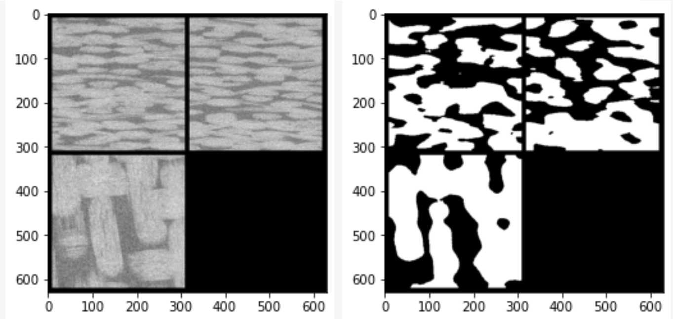
消噪后图片灰度值分布如下
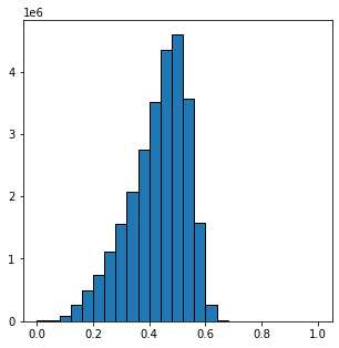
可以看到,灰度值分布并没有像2D图片那样分开为明相和暗相
采用其他过滤器:
start =time.time()
im2 = spim.uniform_filter(im, size=3)
im2 = (im2 - im2.min())/(im2.max() - im2.min())
end = time.time()
print('uniform_filter Running time: %s Seconds'%(end-start))

start =time.time()
im3 = spim.gaussian_filter(im, sigma=1)
im3 = (im3 - im3.min())/(im3.max() - im3.min())
end = time.time()
print('gaussian_filter Running time: %s Seconds'%(end-start))

start =time.time()
im4 = spim.median_filter(im, size=3)
im4 = (im4 - im4.min())/(im4.max() - im4.min())
end = time.time()
print('gaussian_filter Running time: %s Seconds'%(end-start))
fig, ax = subplots(1,3,figsize=[15, 5])
ax[0].hist(im2.flatten(), bins=25, edgecolor='k')
ax[1].hist(im2.flatten(), bins=25, edgecolor='k')
ax[2].hist(im2.flatten(), bins=25, edgecolor='k')
'''
uniform_filter Running time: 0.28285670280456543 Seconds
gaussian_filter Running time: 0.36307644844055176 Seconds
median_filter Running time: 8.655892610549927 Seconds
'''

三种过滤器都没能将骨架和孔隙区分开
#non_local_means.denoise_nl_means()
def denoise_nl_means(image, patch_size=7, patch_distance=11, h=0.1,
                     multichannel=False, fast_mode=True, sigma=0., *,
                     preserve_range=False, channel_axis=None):
    """Perform non-local means denoising on 2D-4D grayscale or RGB images.

    Parameters
    ----------
    image : 2D or 3D ndarray
        Input image to be denoised, which can be 2D or 3D, and grayscale
        or RGB (for 2D images only, see ``multichannel`` parameter). There can
        be any number of channels (does not strictly have to be RGB).
    patch_size : int, optional
        Size of patches used for denoising.
    patch_distance : int, optional
        Maximal distance in pixels where to search patches used for denoising.
    h : float, optional
        Cut-off distance (in gray levels). The higher h, the more permissive
        one is in accepting patches. A higher h results in a smoother image,
        at the expense of blurring features. For a Gaussian noise of standard
        deviation sigma, a rule of thumb is to choose the value of h to be
        sigma of slightly less.
    multichannel : bool, optional
        Whether the last axis of the image is to be interpreted as multiple
        channels or another spatial dimension. This argument is deprecated:
        specify `channel_axis` instead.
    fast_mode : bool, optional
        If True (default value), a fast version of the non-local means
        algorithm is used. If False, the original version of non-local means is
        used. See the Notes section for more details about the algorithms.
    sigma : float, optional
        The standard deviation of the (Gaussian) noise.  If provided, a more
        robust computation of patch weights is computed that takes the expected
        noise variance into account (see Notes below).
    preserve_range : bool, optional
        Whether to keep the original range of values. Otherwise, the input
        image is converted according to the conventions of `img_as_float`.
        Also see https://scikit-image.org/docs/dev/user_guide/data_types.html
    channel_axis : int or None, optional
        If None, the image is assumed to be a grayscale (single channel) image.
        Otherwise, this parameter indicates which axis of the array corresponds
        to channels.

        .. versionadded:: 0.19
           ``channel_axis`` was added in 0.19.

    Returns
    -------
    result : ndarray
        Denoised image, of same shape as `image`.

    Notes
    -----

    The non-local means algorithm is well suited for denoising images with
    specific textures. The principle of the algorithm is to average the value
    of a given pixel with values of other pixels in a limited neighbourhood,
    provided that the *patches* centered on the other pixels are similar enough
    to the patch centered on the pixel of interest.

    In the original version of the algorithm [1]_, corresponding to
    ``fast=False``, the computational complexity is::

        image.size * patch_size ** image.ndim * patch_distance ** image.ndim

    Hence, changing the size of patches or their maximal distance has a
    strong effect on computing times, especially for 3-D images.

    However, the default behavior corresponds to ``fast_mode=True``, for which
    another version of non-local means [2]_ is used, corresponding to a
    complexity of::

        image.size * patch_distance ** image.ndim

    The computing time depends only weakly on the patch size, thanks to
    the computation of the integral of patches distances for a given
    shift, that reduces the number of operations [1]_. Therefore, this
    algorithm executes faster than the classic algorithm
    (``fast_mode=False``), at the expense of using twice as much memory.
    This implementation has been proven to be more efficient compared to
    other alternatives, see e.g. [3]_.

    Compared to the classic algorithm, all pixels of a patch contribute
    to the distance to another patch with the same weight, no matter
    their distance to the center of the patch. This coarser computation
    of the distance can result in a slightly poorer denoising
    performance. Moreover, for small images (images with a linear size
    that is only a few times the patch size), the classic algorithm can
    be faster due to boundary effects.

    The image is padded using the `reflect` mode of `skimage.util.pad`
    before denoising.

    If the noise standard deviation, `sigma`, is provided a more robust
    computation of patch weights is used.  Subtracting the known noise variance
    from the computed patch distances improves the estimates of patch
    similarity, giving a moderate improvement to denoising performance [4]_.
    It was also mentioned as an option for the fast variant of the algorithm in
    [3]_.

    When `sigma` is provided, a smaller `h` should typically be used to
    avoid oversmoothing.  The optimal value for `h` depends on the image
    content and noise level, but a reasonable starting point is
    ``h = 0.8 * sigma`` when `fast_mode` is `True`, or ``h = 0.6 * sigma`` when
    `fast_mode` is `False`.

    References
    ----------
    .. [1] A. Buades, B. Coll, & J-M. Morel. A non-local algorithm for image
           denoising. In CVPR 2005, Vol. 2, pp. 60-65, IEEE.
           :DOI:`10.1109/CVPR.2005.38`

    .. [2] J. Darbon, A. Cunha, T.F. Chan, S. Osher, and G.J. Jensen, Fast
           nonlocal filtering applied to electron cryomicroscopy, in 5th IEEE
           International Symposium on Biomedical Imaging: From Nano to Macro,
           2008, pp. 1331-1334.
           :DOI:`10.1109/ISBI.2008.4541250`

    .. [3] Jacques Froment. Parameter-Free Fast Pixelwise Non-Local Means
           Denoising. Image Processing On Line, 2014, vol. 4, pp. 300-326.
           :DOI:`10.5201/ipol.2014.120`

    .. [4] A. Buades, B. Coll, & J-M. Morel. Non-Local Means Denoising.
           Image Processing On Line, 2011, vol. 1, pp. 208-212.
           :DOI:`10.5201/ipol.2011.bcm_nlm`

    Examples
    --------
    >>> a = np.zeros((40, 40))
    >>> a[10:-10, 10:-10] = 1.
    >>> rng = np.random.default_rng()
    >>> a += 0.3 * rng.standard_normal(a.shape)
    >>> denoised_a = denoise_nl_means(a, 7, 5, 0.1)
    """
1.3 生成孔隙网络模型
基于SNOW算法提取孔隙网络模型
from porespy.filters import find_peaks, trim_saddle_points, trim_nearby_peaks
from porespy.tools import randomize_colors
from skimage.segmentation import watershed
sigma = 0.4
dt = spim.distance_transform_edt(input=(im1 0)
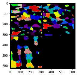
regions = randomize_colors(regions)#赋予不同孔隙区域不同的颜色
fig, ax = plt.subplots()
ax.imshow(ps.visualization.show_planes(regions), cmap=plt.cm.nipy_spectral);
#将分割过的区域等效成球棒模型
import openpnm as op
net = ps.networks.regions_to_network(regions, voxel_size=1)
#提取的PNM数据可以直接导入OpenPNM
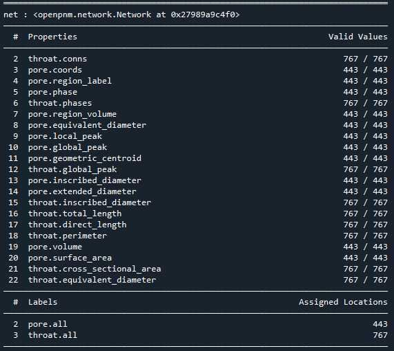
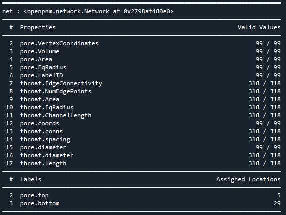
pn = op.io.network_from_porespy(net)
print(pn)
ax = op.visualization.plot_coordinates(pn)
ax = op.visualization.plot_connections(pn, ax=ax)
def regions_to_network(regions, phases=None, voxel_size=1, accuracy='standard'):
    r"""
    Analyzes an image that has been partitioned into pore regions and extracts
    the pore and throat geometry as well as network connectivity.

    Parameters
    ----------
    regions : ndarray
        An image of the material partitioned into individual regions.
        Zeros in this image are ignored.
    phases : ndarray, optional
        An image indicating to which phase each voxel belongs. The returned
        network contains a 'pore.phase' array with the corresponding value.
        If not given a value of 1 is assigned to every pore.
    voxel_size : scalar (default = 1)
        The resolution of the image, expressed as the length of one side of a
        voxel, so the volume of a voxel would be **voxel_size**-cubed.
    accuracy : string
        Controls how accurately certain properties are calculated. Options are:

        'standard' (default)
            Computes the surface areas and perimeters by simply counting
            voxels.  This is *much* faster but does not properly account
            for the rough, voxelated nature of the surfaces.
        'high'
            Computes surface areas using the marching cube method, and
            perimeters using the fast marching method.  These are substantially
            slower but better account for the voxelated nature of the images.

    Returns
    -------
    net : dict
        A dictionary containing all the pore and throat size data, as well as
        the network topological information.  The dictionary names use the
        OpenPNM convention (i.e. 'pore.coords', 'throat.conns').

    Notes
    -----
    The meaning of each of the values returned in ``net`` are outlined below:

    'pore.region_label'
        The region labels corresponding to the watershed extraction. The
        pore indices and regions labels will be offset by 1, so pore 0
        will be region 1.
    'throat.conns'
        An *Nt-by-2* array indicating which pores are connected to each other
    'pore.region_label'
        Mapping of regions in the watershed segmentation to pores in the
        network
    'pore.local_peak'
        The coordinates of the location of the maxima of the distance transform
        performed on the pore region in isolation
    'pore.global_peak'
        The coordinates of the location of the maxima of the distance transform
        performed on the full image
    'pore.geometric_centroid'
        The center of mass of the pore region as calculated by
        ``skimage.measure.center_of_mass``
    'throat.global_peak'
        The coordinates of the location of the maxima of the distance transform
        performed on the full image
    'pore.region_volume'
        The volume of the pore region computed by summing the voxels
    'pore.volume'
        The volume of the pore found by as volume of a mesh obtained from the
        marching cubes algorithm
    'pore.surface_area'
        The surface area of the pore region as calculated by either counting
        voxels or using the fast marching method to generate a tetramesh (if
        ``accuracy`` is set to ``'high'``.)
    'throat.cross_sectional_area'
        The cross-sectional area of the throat found by either counting
        voxels or using the fast marching method to generate a tetramesh (if
        ``accuracy`` is set to ``'high'``.)
    'throat.perimeter'
        The perimeter of the throat found by counting voxels on the edge of
        the region defined by the intersection of two regions.
    'pore.inscribed_diameter'
        The diameter of the largest sphere inscribed in the pore region. This
        is found as the maximum of the distance transform on the region in
        isolation.
    'pore.extended_diameter'
        The diamter of the largest sphere inscribed in overal image, which
        can extend outside the pore region. This is found as the local maximum
        of the distance transform on the full image.
    'throat.inscribed_diameter'
        The diameter of the largest sphere inscribed in the throat.  This
        is found as the local maximum of the distance transform in the area
        where to regions meet.
    'throat.total_length'
        The length between pore centered via the throat center
    'throat.direct_length'
        The length between two pore centers on a straight line between them
        that does not pass through the throat centroid.

    Examples
    --------
    `Click here
    `_
    to view online example.

    """
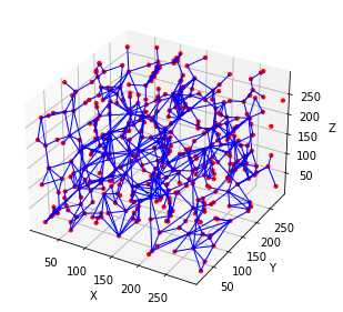
相比Avizo最大球法提取的孔隙网络模型:
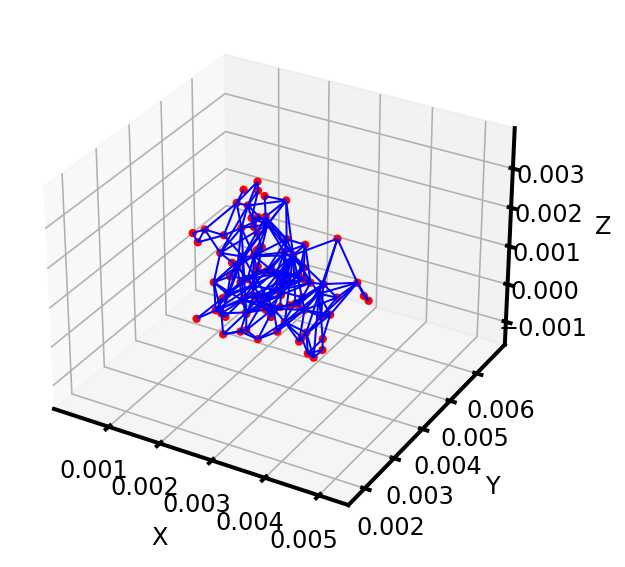
可以看到,poreSpy提取的孔隙网络模型中无论孔隙还是流道数量都远高于Avizo提取的模型,造成这个区别的原因可能是Avizo提取PNM过程中有去除孤立孔隙的步骤,从poreSpy提取的PNM图形上也可以看到许多孤立孔隙,目前在PoreSpy上没找到去除孤立孔隙的方法
2. 问题(待解决)
- 图像处理相关的原理我还没弄明白,比如噪声过滤的那几个过滤器我不知道是怎么运转的,为什么2D图片消噪效果很好但到了3D就不行
- 关于SNOW算法,我看了那篇文献,里面有几个关于怎么用代码实现网络提取的补充材料我这边搞不到,PoreSpy里的注释感觉不够详细,还是不知道那几行代码的原理,文献链接如下:>Phys. Rev. E 96, 023307 (2017) - Versatile and efficient pore network extraction method using marker-based watershed segmentation (aps.org), 补充材料见 Supplemental Material at http://link.aps.org/supplemental/10.1103/PhysRevE.96.023307 for the source code of the algorithm
- 关于孤立孔隙的去除,这个我没找到PoreSpy里有相关的介绍,SNOW算法的文献里也没有
Comments NOTHING