[PoreSpy] 图像导入和基本处理
1 图像导入
1.1 2D图像
CT扫描的图像是连续的二维切片,将这些图片放进一个文件夹里,通过特定的Python函数可以导入,
import imageio.v2 as imageio
import porespy as ps
import numpy as np
from skimage.io import imread_collection
from matplotlib.pyplot import subplots
seq = io.imread_collection("C:/Users/ALPHA/Desktop/PNM\object/test3-2d/*.tif") #读取文件夹里的tif文件并以列表的方式存储
seq.files

'''
['C:/Users/ALPHA/Desktop/PNM/object/test3-2d\\test3-2D000.tif',
 'C:/Users/ALPHA/Desktop/PNM/object/test3-2d\\test3-2D001.tif',
 'C:/Users/ALPHA/Desktop/PNM/object/test3-2d\\test3-2D002.tif',
 .....
 'C:/Users/ALPHA/Desktop/PNM/object/test3-2d\\test3-2D297.tif',
 'C:/Users/ALPHA/Desktop/PNM/object/test3-2d\\test3-2D298.tif',
 'C:/Users/ALPHA/Desktop/PNM/object/test3-2d\\test3-2D299.tif']
'''
def imread_collection(load_pattern, conserve_memory=True,
                      plugin=None, **plugin_args):
    """
    Load a collection of images.

    Parameters
    ----------
    load_pattern : str or list
        List of objects to load. These are usually filenames, but may
        vary depending on the currently active plugin.  See the docstring
        for ``ImageCollection`` for the default behaviour of this parameter.
    conserve_memory : bool, optional
        If True, never keep more than one in memory at a specific
        time.  Otherwise, images will be cached once they are loaded.

    Returns
    -------
    ic : ImageCollection
        Collection of images.

    Other Parameters
    ----------------
    plugin_args : keywords
        Passed to the given plugin.

    """
现在可以从列表中调取任意的图像进行可视化
fig, ax = subplots(figsize=[5, 5])
im1=seq[0]
ax.imshow(im1,cmap='gray');
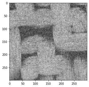
图片以灰度图的形式显示,即每个像素点都有一个对应的灰度值,Python中将图片的所有灰度值储存为一个数组:
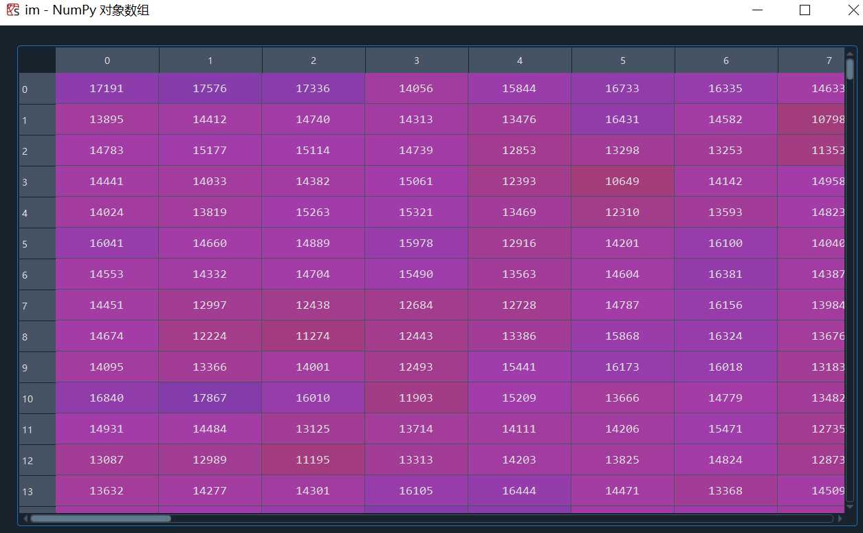
这里的灰度值是16bit,平时所说的0-255的灰度值是8bit,换算一下即可,具体区别可以参考:
(4条消息) 如何理解图像深度:8bit、16bit、24bit、32bit; 16.7M色彩_图片位深度_WaitFoF的博客-CSDN博客
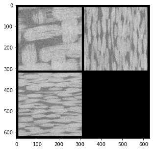
1.2 2D文件夹转3D文件
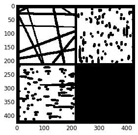
我们可以通过下面的代码将连续二维切片文件转换为单一的三维图片
#遍历文件夹中的所有切片,取每个切片的xz,yz面,合并成整个模型的xz,yz面,得到模型的三维图片
im3d = np.zeros([*seq[0].shape, len(seq)])
for i, im in enumerate(seq):
    im3d[..., i] = im
fig, ax = subplots(figsize=[5, 5])
ax.imshow(ps.visualization.show_planes(im3d),cmap='gray');
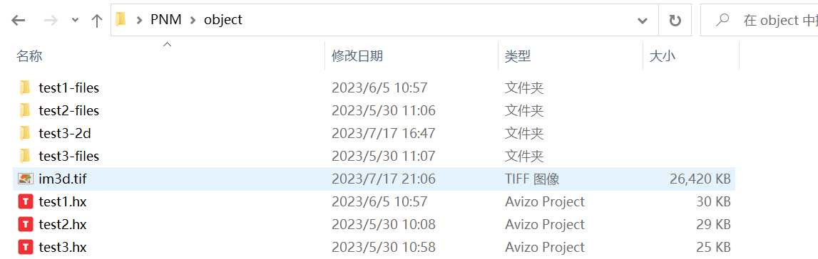
将生成的3D图像存储起来
imageio.volsave('C:/Users/ALPHA/Desktop/PNM/object/im3d.tif',np.array(im3d, dtype=np.int8))
#volsave = volwrite
def volwrite(uri, im, format=None, **kwargs):
    """volwrite(uri, vol, format=None, **kwargs)

    Write a volume to the specified file.

    Parameters
    ----------
    uri : {str, pathlib.Path, file}
        The resource to write the image to, e.g. a filename, pathlib.Path
        or file object, see the docs for more info.
    vol : numpy.ndarray
        The image data. Must be NxMxL (or NxMxLxK if each voxel is a tuple).
    format : str
        The format to use to read the file. By default imageio selects
        the appropriate for you based on the filename and its contents.
    kwargs : ...
        Further keyword arguments are passed to the writer. See :func:`.help`
        to see what arguments are available for a particular format.
    """
1.2 直接导入3D图像
im2 = imageio.volread('C:/Users/ALPHA/Desktop/PNM/object/test3-3D.tif')
ps.imshow(im2, axis=0,cmap='gray');

def volread(uri, format=None, **kwargs):
    """volread(uri, format=None, **kwargs)

    Reads a volume from the specified file. Returns a numpy array, which
    comes with a dict of meta data at its 'meta' attribute.

    Parameters
    ----------
    uri : {str, pathlib.Path, bytes, file}
        The resource to load the volume from, e.g. a filename, pathlib.Path,
        http address or file object, see the docs for more info.
    format : str
        The format to use to read the file. By default imageio selects
        the appropriate for you based on the filename and its contents.
    kwargs : ...
        Further keyword arguments are passed to the reader. See :func:`.help`
        to see what arguments are available for a particular format.
    """
2 图像处理
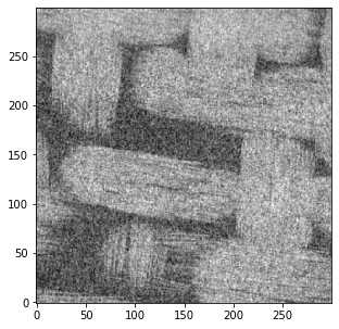
CT产生的图像都是灰度值图象的,每个像素都包含一个数值,指示该位置的强度。在理想的图片中,灰度值将很好地分布,使得对应于固体框架的所有明亮像素都具有高灰度值(即200-255),而对应于孔隙的所有暗像素都具有低灰度值值(即0-50)。如果是这种情况,区分或分割固体和孔隙隙将非常容易。在PoreSpy和imageio里图像为灰度值图像,以储存
2.1 图像的噪声
在分割固体和孔隙的过程中需要对CT图像进行降噪处理,下面简单说一下什么是‘噪声’
先生成一个随机的图片
import imageio.v2 as imageio
import porespy as ps
import numpy as np
from matplotlib.pyplot import subplots
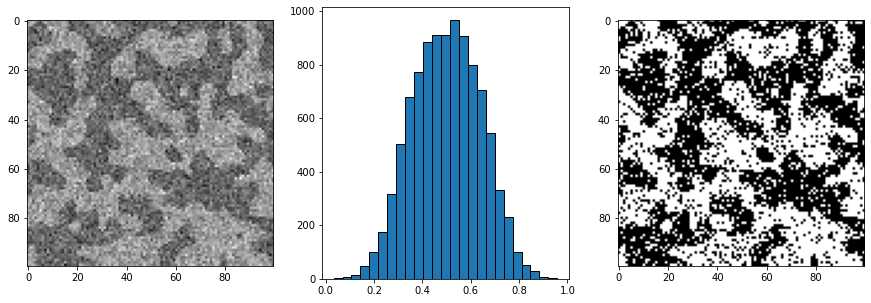
im = ps.generators.blobs(shape=[100, 100])
new_im = (im*0.2) * np.random.rand(*im.shape) + 0.8*im
new_im += (~im*0.2) * np.random.rand(*im.shape)
fig, ax = subplots(figsize=[5, 5])
ax.imshow(new_im,cmap='gray');
#ps.generators.blobs()
def blobs(
    shape: List[int],
    porosity: float = 0.5,
    blobiness: int = 1,
    divs: int = 1,
    seed=None,
):
    """
    Generates an image containing amorphous blobs

    Parameters
    ----------
    shape : list
        The size of the image to generate in [Nx, Ny, Nz] where N is the
        number of voxels
    porosity : float
        If specified, this will threshold the image to the specified value
        prior to returning.  If ``None`` is specified, then the scalar
        noise field is converted to a uniform distribution and returned
        without thresholding.
    blobiness : int or list of ints(default = 1)
        Controls the morphology of the blobs.  A higher number results in
        a larger number of small blobs.  If a list is supplied then the
        blobs are anisotropic.
    divs : int or array_like
        The number of times to divide the image for parallel processing.
        If ``1`` then parallel processing does not occur.  ``2`` is
        equivalent to ``[2, 2, 2]`` for a 3D image.  The number of cores
        used is specified in ``porespy.settings.ncores`` and defaults to
        all cores.
    seed : int, optional, default = `None`
        Initializes numpy's random number generator to the specified state. If not
        provided, the current global value is used. This means calls to
        ``np.random.state(seed)`` prior to calling this function will be respected.

    Returns
    -------
    image : ndarray
        A boolean array with ``True`` values denoting the pore space

    See Also
    --------
    norm_to_uniform

    Notes
    -----
    This function generates random noise, the applies a gaussian blur to
    the noise with a sigma controlled by the blobiness argument as:

        $$ np.mean(shape) / (40 * blobiness) $$

    The value of 40 was chosen so that a ``blobiness`` of 1 gave a
    reasonable result.

    Examples
    --------
    `Click here
    `_
    to view online example.

    """
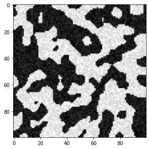
可以看出在固体框架(白色区域)内存在一些较黑的点,孔隙(黑色区域)内存在一些较白的点,这些本不该存在的点就是‘’噪声‘’
根据灰度值我们可以画一个直方图来观察上面图像中像素点的灰度分布
fig, ax = subplots(figsize=[5, 5])
ax.hist(new_im.flatten(), bins=25, edgecolor='k');
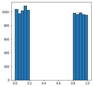
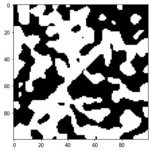
可以看到看到,所有值小于0.5的像素都属于暗相,而其他像素属于亮相。设置一个简单的全局阈值可以完美地解决噪声再现原始图像:
fig, ax = subplots(figsize=[5, 5])
ax.imshow(new_im > 0.5,cmap='gray');
现在看一个更真实的噪声分布,:
new_im = np.random.normal(loc=.4, scale=0.1, size=im.shape) * im
new_im += np.random.normal(loc=.6, scale=0.1, size=im.shape) * (~im)
fig, ax = subplots(1, 3, figsize=[15, 5])
ax[0].imshow(new_im)
ax[1].hist(new_im.flatten(), bins=25, edgecolor='k')
ax[2].imshow(new_im > 0.5);
2.2 噪声过滤
描述上述噪声的最简单方式是,我们知道位于黑暗区域的某些像素的强度值比我们知道位于明亮区域的某些像素更亮,反之亦然。这会导致在应用阈值时错误标记像素。
我们的眼睛仍然可以看到黑暗和明亮的区域,消除噪点的原因是黑暗区域中大多数像素比明亮区域暗,反之亦然。我们的眼睛可以对数据进行某种平均,以丢弃或校正杂散强度的像素。
2.2.1 不保留边缘的过滤方式
因此,可以考虑将每个像素替换为一个值,该值是其周围像素灰度的平均值。我们可以对灰度值直接平均,或者用高斯模糊这样的加权平均:
import scipy.ndimage as spim
im = imageio.volread('C:/Users/ALPHA/Desktop/PNM\object/test3-2d/test3-2D000.tif')
im = (im - im.min())/(im.max() - im.min())

im1 = spim.uniform_filter(im, size=3)
im1 = (im1 - im1.min())/(im1.max() - im1.min())
im2 = spim.gaussian_filter(im, sigma=1)
im2 = (im2 - im2.min())/(im2.max() - im2.min())
fig, ax = subplots(2, 3, figsize=[10, 5])
ax[0][0].imshow(im,cmap='gray')
ax[0][1].imshow(im1,cmap='gray')
ax[0][2].imshow(im2,cmap='gray')
ax[1][0].imshow(im > 0.6,cmap='gray')
ax[1][1].imshow(im1 > 0.6,cmap='gray')
ax[1][2].imshow(im2 > 0.6,cmap='gray');
#spim.uniform_filter()
def uniform_filter(input, size=3, output=None, mode="reflect",
                   cval=0.0, origin=0, *, axes=None):
    """Multidimensional uniform filter.

    Parameters
    ----------
    %(input)s
    size : int or sequence of ints, optional
        The sizes of the uniform filter are given for each axis as a
        sequence, or as a single number, in which case the size is
        equal for all axes.
    %(output)s
    %(mode_multiple)s
    %(cval)s
    %(origin_multiple)s
    axes : tuple of int or None, optional
        If None, `input` is filtered along all axes. Otherwise,
        `input` is filtered along the specified axes. When `axes` is
        specified, any tuples used for `size`, `origin`, and/or `mode`
        must match the length of `axes`. The ith entry in any of these tuples
        corresponds to the ith entry in `axes`.

    Returns
    -------
    uniform_filter : ndarray
        Filtered array. Has the same shape as `input`.

    Notes
    -----
    The multidimensional filter is implemented as a sequence of
    1-D uniform filters. The intermediate arrays are stored
    in the same data type as the output. Therefore, for output types
    with a limited precision, the results may be imprecise because
    intermediate results may be stored with insufficient precision.

    Examples
    --------
    >>> from scipy import ndimage, datasets
    >>> import matplotlib.pyplot as plt
    >>> fig = plt.figure()
    >>> plt.gray()  # show the filtered result in grayscale
    >>> ax1 = fig.add_subplot(121)  # left side
    >>> ax2 = fig.add_subplot(122)  # right side
    >>> ascent = datasets.ascent()
    >>> result = ndimage.uniform_filter(ascent, size=20)
    >>> ax1.imshow(ascent)
    >>> ax2.imshow(result)
    >>> plt.show()
    """
#spim.gaussian_filter()
def gaussian_filter(input, sigma, order=0, output=None,
                    mode="reflect", cval=0.0, truncate=4.0, *, radius=None,
                    axes=None):
    """Multidimensional Gaussian filter.

    Parameters
    ----------
    %(input)s
    sigma : scalar or sequence of scalars
        Standard deviation for Gaussian kernel. The standard
        deviations of the Gaussian filter are given for each axis as a
        sequence, or as a single number, in which case it is equal for
        all axes.
    order : int or sequence of ints, optional
        The order of the filter along each axis is given as a sequence
        of integers, or as a single number. An order of 0 corresponds
        to convolution with a Gaussian kernel. A positive order
        corresponds to convolution with that derivative of a Gaussian.
    %(output)s
    %(mode_multiple)s
    %(cval)s
    truncate : float, optional
        Truncate the filter at this many standard deviations.
        Default is 4.0.
    radius : None or int or sequence of ints, optional
        Radius of the Gaussian kernel. The radius are given for each axis
        as a sequence, or as a single number, in which case it is equal
        for all axes. If specified, the size of the kernel along each axis
        will be ``2*radius + 1``, and `truncate` is ignored.
        Default is None.
    axes : tuple of int or None, optional
        If None, `input` is filtered along all axes. Otherwise,
        `input` is filtered along the specified axes. When `axes` is
        specified, any tuples used for `sigma`, `order`, `mode` and/or `radius`
        must match the length of `axes`. The ith entry in any of these tuples
        corresponds to the ith entry in `axes`.

    Returns
    -------
    gaussian_filter : ndarray
        Returned array of same shape as `input`.

    Notes
    -----
    The multidimensional filter is implemented as a sequence of
    1-D convolution filters. The intermediate arrays are
    stored in the same data type as the output. Therefore, for output
    types with a limited precision, the results may be imprecise
    because intermediate results may be stored with insufficient
    precision.

    The Gaussian kernel will have size ``2*radius + 1`` along each axis. If
    `radius` is None, the default ``radius = round(truncate * sigma)`` will be
    used.

    Examples
    --------
    >>> from scipy.ndimage import gaussian_filter
    >>> import numpy as np
    >>> a = np.arange(50, step=2).reshape((5,5))
    >>> a
    array([[ 0,  2,  4,  6,  8],
           [10, 12, 14, 16, 18],
           [20, 22, 24, 26, 28],
           [30, 32, 34, 36, 38],
           [40, 42, 44, 46, 48]])
    >>> gaussian_filter(a, sigma=1)
    array([[ 4,  6,  8,  9, 11],
           [10, 12, 14, 15, 17],
           [20, 22, 24, 25, 27],
           [29, 31, 33, 34, 36],
           [35, 37, 39, 40, 42]])

    >>> from scipy import datasets
    >>> import matplotlib.pyplot as plt
    >>> fig = plt.figure()
    >>> plt.gray()  # show the filtered result in grayscale
    >>> ax1 = fig.add_subplot(121)  # left side
    >>> ax2 = fig.add_subplot(122)  # right side
    >>> ascent = datasets.ascent()
    >>> result = gaussian_filter(ascent, sigma=5)
    >>> ax1.imshow(ascent)
    >>> ax2.imshow(result)
    >>> plt.show()
    """
gaussian 高斯滤波原理可参考:高斯滤波gaussian_filter()_gaussian filter_wanghua609的博客-CSDN博客
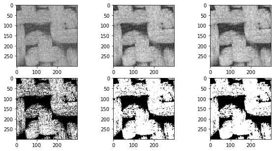
上述结果还不错,但如本小节标题中所述,这些过滤器不会保留边缘。可能上面织物的照片显示的不太明显,考虑以下人为情况:
im = ~ps.generators.random_spheres([100, 100], r=8)*1.0
im1 = spim.uniform_filter(im, size=6)
im2 = spim.gaussian_filter(im, sigma=2)
fig, ax = subplots(2, 2, figsize=[10, 10])
ax[0][0].imshow(im1,cmap='gray')
ax[0][1].imshow(im2,cmap='gray')
ax[1][0].imshow(im1 > im1.mean(),cmap='gray')
ax[1][1].imshow(im2 > im2.mean(),cmap='gray');
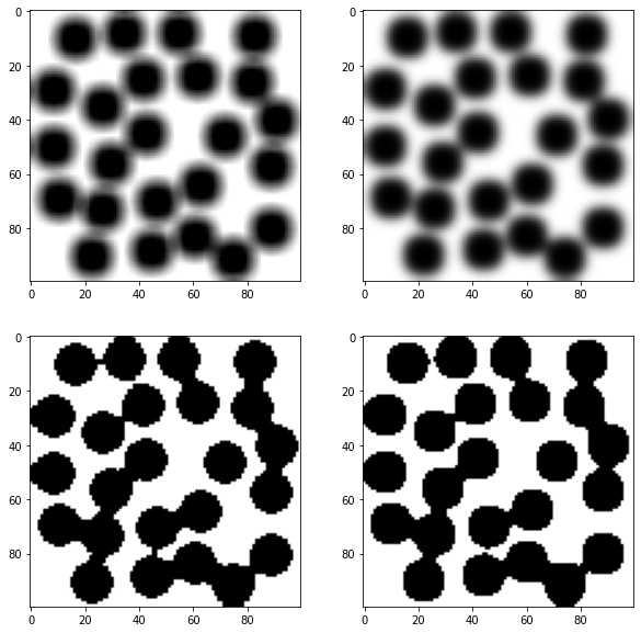
在上面的图中可以看到,应用阈值后分割效果不太好,有部分未连通的孔隙在分割之后连在一块了。原因是过滤器合并了来自整个图片的灰度值,孔隙与固体相之间的灰度值分割不准确,所以看孔隙的边缘比较模糊。
2.2.2 保留边缘的过滤方式
import imageio.v2 as imageio
import porespy as ps
import numpy as np
from matplotlib.pyplot import subplots
import scipy.ndimage as spim
from skimage.restoration import non_local_means, estimate_sigma
im = imageio.volread('C:/Users/ALPHA/Desktop/PNM\object/test3-2d/test3-2D000.tif')
im = (im - im.min())/(im.max() - im.min())
im1 = spim.median_filter(im, size=3)
im1 = (im1 - im1.min())/(im1.max() - im1.min())
s = estimate_sigma(im)
im2 = non_local_means.denoise_nl_means(im)
im2 = (im2 - im2.min())/(im2.max() - im2.min())
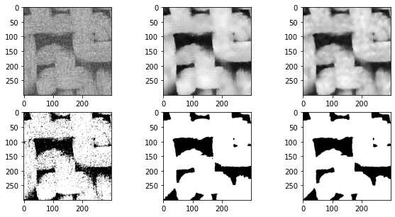
fig, ax = subplots(2, 3, figsize=[10, 5])
ax[0][0].imshow(im,cmap='gray')
ax[0][1].imshow(im1,cmap='gray')
ax[0][2].imshow(im2,cmap='gray')
ax[1][0].imshow(im > 0.6,cmap='gray')
ax[1][1].imshow(im1 > 0.6,cmap='gray')
ax[1][2].imshow(im2 > 0.5,cmap='gray');
def median_filter(input, size=None, footprint=None, output=None,
                  mode="reflect", cval=0.0, origin=0, *, axes=None):
    """
    Calculate a multidimensional median filter.

    Parameters
    ----------
    %(input)s
    %(size_foot)s
    %(output)s
    %(mode_reflect)s
    %(cval)s
    %(origin_multiple)s
    axes : tuple of int or None, optional
        If None, `input` is filtered along all axes. Otherwise,
        `input` is filtered along the specified axes.

    Returns
    -------
    median_filter : ndarray
        Filtered array. Has the same shape as `input`.

    See Also
    --------
    scipy.signal.medfilt2d

    Notes
    -----
    For 2-dimensional images with ``uint8``, ``float32`` or ``float64`` dtypes
    the specialised function `scipy.signal.medfilt2d` may be faster. It is
    however limited to constant mode with ``cval=0``.

    Examples
    --------
    >>> from scipy import ndimage, datasets
    >>> import matplotlib.pyplot as plt
    >>> fig = plt.figure()
    >>> plt.gray()  # show the filtered result in grayscale
    >>> ax1 = fig.add_subplot(121)  # left side
    >>> ax2 = fig.add_subplot(122)  # right side
    >>> ascent = datasets.ascent()
    >>> result = ndimage.median_filter(ascent, size=20)
    >>> ax1.imshow(ascent)
    >>> ax2.imshow(result)
    >>> plt.show()
    """
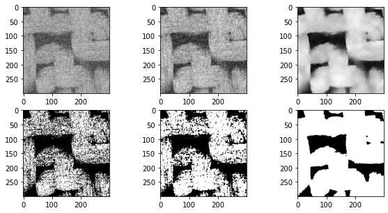
在上面的图片中,中间的图像显示了中值过滤器,边缘明显不那么模糊,而不是上一节中使用的高斯和均匀滤波器。阈值后的结果也更好。上面的右列显示了非局部均值过滤器,结果明显更优越。下面尝试优化各种可调参数:
fig, ax = subplots(1, 3, figsize=[15, 5])
ax[0].hist(im.flatten(), bins=25, edgecolor='k')
ax[1].hist(im1.flatten(), bins=25, edgecolor='k')
ax[2].hist(im2.flatten(), bins=25, edgecolor='k');
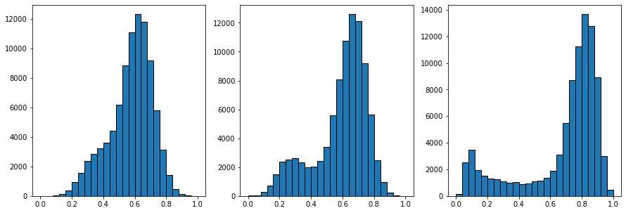
上面的三个直方图显示了过滤前、中值过滤器之后和非局部均值过滤器之后的像素值分布。非局部均值直方图右侧的峰是明亮的像素,现在已经与黑暗的像素分开。
im = imageio.volread('C:/Users/ALPHA/Desktop/PNM\object/test3-2d/test3-2D000.tif')
im = (im - im.min())/(im.max() - im.min())
s = estimate_sigma(im)
kw = {
'patch_size': 7,
'patch_distance': 11,
'h': 0.1,
}
im1 = non_local_means.denoise_nl_means(im, sigma=s, **kw)
im1 = (im1 - im1.min())/(im1.max() - im1.min())
kw = {
'patch_size': 7,
'patch_distance': 7,
'h': 0.1,
}
im2 = non_local_means.denoise_nl_means(im, sigma=s, **kw)
im2 = (im2 - im2.min())/(im2.max() - im2.min())
kw = {
'patch_size': 9,
'patch_distance': 7,
'h': 0.1,
}
im3 = non_local_means.denoise_nl_means(im, sigma=s, **kw)
im3 = (im3 - im3.min())/(im3.max() - im3.min())
fig, ax = subplots(2, 3, figsize=[10, 5])
ax[0][0].imshow(im,cmap='gray')
ax[0][1].imshow(im1,cmap='gray')
ax[0][2].imshow(im2,cmap='gray')
ax[1][0].imshow(im > 0.5,cmap='gray')
ax[1][1].imshow(im1 > 0.5,cmap='gray')
ax[1][2].imshow(im2 > 0.5,cmap='gray');
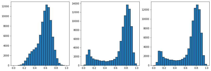
fig, ax = subplots(1, 3, figsize=[15, 5])
ax[0].hist(im.flatten(), bins=25, edgecolor='k')
ax[1].hist(im1.flatten(), bins=25, edgecolor='k')
ax[2].hist(im2.flatten(), bins=25, edgecolor='k');
#estimate_sigma
def estimate_sigma(image, average_sigmas=False, multichannel=False, *,
                   channel_axis=None):
    """
    Robust wavelet-based estimator of the (Gaussian) noise standard deviation.

    Parameters
    ----------
    image : ndarray
        Image for which to estimate the noise standard deviation.
    average_sigmas : bool, optional
        If true, average the channel estimates of `sigma`.  Otherwise return
        a list of sigmas corresponding to each channel.
    multichannel : bool
        Estimate sigma separately for each channel. This argument is
        deprecated: specify `channel_axis` instead.
    channel_axis : int or None, optional
        If None, the image is assumed to be a grayscale (single channel) image.
        Otherwise, this parameter indicates which axis of the array corresponds
        to channels.

        .. versionadded:: 0.19
           ``channel_axis`` was added in 0.19.

    Returns
    -------
    sigma : float or list
        Estimated noise standard deviation(s).  If `multichannel` is True and
        `average_sigmas` is False, a separate noise estimate for each channel
        is returned.  Otherwise, the average of the individual channel
        estimates is returned.

    Notes
    -----
    This function assumes the noise follows a Gaussian distribution. The
    estimation algorithm is based on the median absolute deviation of the
    wavelet detail coefficients as described in section 4.2 of [1]_.

    References
    ----------
    .. [1] D. L. Donoho and I. M. Johnstone. "Ideal spatial adaptation
       by wavelet shrinkage." Biometrika 81.3 (1994): 425-455.
       :DOI:`10.1093/biomet/81.3.425`

    Examples
    --------
    >>> import skimage.data
    >>> from skimage import img_as_float
    >>> img = img_as_float(skimage.data.camera())
    >>> sigma = 0.1
    >>> rng = np.random.default_rng()
    >>> img = img + sigma * rng.standard_normal(img.shape)
    >>> sigma_hat = estimate_sigma(img, channel_axis=None)
#non_local_means.denoise_nl_means()
def denoise_nl_means(image, patch_size=7, patch_distance=11, h=0.1,
                     multichannel=False, fast_mode=True, sigma=0., *,
                     preserve_range=False, channel_axis=None):
    """Perform non-local means denoising on 2D-4D grayscale or RGB images.

    Parameters
    ----------
    image : 2D or 3D ndarray
        Input image to be denoised, which can be 2D or 3D, and grayscale
        or RGB (for 2D images only, see ``multichannel`` parameter). There can
        be any number of channels (does not strictly have to be RGB).
    patch_size : int, optional
        Size of patches used for denoising.
    patch_distance : int, optional
        Maximal distance in pixels where to search patches used for denoising.
    h : float, optional
        Cut-off distance (in gray levels). The higher h, the more permissive
        one is in accepting patches. A higher h results in a smoother image,
        at the expense of blurring features. For a Gaussian noise of standard
        deviation sigma, a rule of thumb is to choose the value of h to be
        sigma of slightly less.
    multichannel : bool, optional
        Whether the last axis of the image is to be interpreted as multiple
        channels or another spatial dimension. This argument is deprecated:
        specify `channel_axis` instead.
    fast_mode : bool, optional
        If True (default value), a fast version of the non-local means
        algorithm is used. If False, the original version of non-local means is
        used. See the Notes section for more details about the algorithms.
    sigma : float, optional
        The standard deviation of the (Gaussian) noise.  If provided, a more
        robust computation of patch weights is computed that takes the expected
        noise variance into account (see Notes below).
    preserve_range : bool, optional
        Whether to keep the original range of values. Otherwise, the input
        image is converted according to the conventions of `img_as_float`.
        Also see https://scikit-image.org/docs/dev/user_guide/data_types.html
    channel_axis : int or None, optional
        If None, the image is assumed to be a grayscale (single channel) image.
        Otherwise, this parameter indicates which axis of the array corresponds
        to channels.

        .. versionadded:: 0.19
           ``channel_axis`` was added in 0.19.

    Returns
    -------
    result : ndarray
        Denoised image, of same shape as `image`.

    Notes
    -----

    The non-local means algorithm is well suited for denoising images with
    specific textures. The principle of the algorithm is to average the value
    of a given pixel with values of other pixels in a limited neighbourhood,
    provided that the *patches* centered on the other pixels are similar enough
    to the patch centered on the pixel of interest.

    In the original version of the algorithm [1]_, corresponding to
    ``fast=False``, the computational complexity is::

        image.size * patch_size ** image.ndim * patch_distance ** image.ndim

    Hence, changing the size of patches or their maximal distance has a
    strong effect on computing times, especially for 3-D images.

    However, the default behavior corresponds to ``fast_mode=True``, for which
    another version of non-local means [2]_ is used, corresponding to a
    complexity of::

        image.size * patch_distance ** image.ndim

    The computing time depends only weakly on the patch size, thanks to
    the computation of the integral of patches distances for a given
    shift, that reduces the number of operations [1]_. Therefore, this
    algorithm executes faster than the classic algorithm
    (``fast_mode=False``), at the expense of using twice as much memory.
    This implementation has been proven to be more efficient compared to
    other alternatives, see e.g. [3]_.

    Compared to the classic algorithm, all pixels of a patch contribute
    to the distance to another patch with the same weight, no matter
    their distance to the center of the patch. This coarser computation
    of the distance can result in a slightly poorer denoising
    performance. Moreover, for small images (images with a linear size
    that is only a few times the patch size), the classic algorithm can
    be faster due to boundary effects.

    The image is padded using the `reflect` mode of `skimage.util.pad`
    before denoising.

    If the noise standard deviation, `sigma`, is provided a more robust
    computation of patch weights is used.  Subtracting the known noise variance
    from the computed patch distances improves the estimates of patch
    similarity, giving a moderate improvement to denoising performance [4]_.
    It was also mentioned as an option for the fast variant of the algorithm in
    [3]_.

    When `sigma` is provided, a smaller `h` should typically be used to
    avoid oversmoothing.  The optimal value for `h` depends on the image
    content and noise level, but a reasonable starting point is
    ``h = 0.8 * sigma`` when `fast_mode` is `True`, or ``h = 0.6 * sigma`` when
    `fast_mode` is `False`.

    References
    ----------
    .. [1] A. Buades, B. Coll, & J-M. Morel. A non-local algorithm for image
           denoising. In CVPR 2005, Vol. 2, pp. 60-65, IEEE.
           :DOI:`10.1109/CVPR.2005.38`

    .. [2] J. Darbon, A. Cunha, T.F. Chan, S. Osher, and G.J. Jensen, Fast
           nonlocal filtering applied to electron cryomicroscopy, in 5th IEEE
           International Symposium on Biomedical Imaging: From Nano to Macro,
           2008, pp. 1331-1334.
           :DOI:`10.1109/ISBI.2008.4541250`

    .. [3] Jacques Froment. Parameter-Free Fast Pixelwise Non-Local Means
           Denoising. Image Processing On Line, 2014, vol. 4, pp. 300-326.
           :DOI:`10.5201/ipol.2014.120`

    .. [4] A. Buades, B. Coll, & J-M. Morel. Non-Local Means Denoising.
           Image Processing On Line, 2011, vol. 1, pp. 208-212.
           :DOI:`10.5201/ipol.2011.bcm_nlm`

    Examples
    --------
    >>> a = np.zeros((40, 40))
    >>> a[10:-10, 10:-10] = 1.
    >>> rng = np.random.default_rng()
    >>> a += 0.3 * rng.standard_normal(a.shape)
    >>> denoised_a = denoise_nl_means(a, 7, 5, 0.1)
    """
2.3 孔隙区域分割
步骤如下:
Distance Transforms二值图像的距离变换 >() Distance Transforms二值图像的距离变换及其应用_HuiYu-Li的博客-CSDN博客
Distance Transforms Peaks 峰值提取
孔隙区域划分
PoreSpy包含一个预定的函数SNOW算法,能够自动应用所有步骤,现在在3D图像上说明各个步骤。
SNOW(subnetwork of the oversegmented watershed)算法基于标记流域的分割算法将图像划分为属于每个孔隙的区域。SNOW 算法的主要贡献是在图像中找到一组合适的初始标记,以便分水岭不会过度分割。
分水岭算法-watershed 详情可参考:图像分割的经典算法:分水岭算法 - 知乎 (zhihu.com)
- 1、导入包
import imageio
import numpy as np
import porespy as ps
import openpnm as op
import scipy.ndimage as spim
import matplotlib.pyplot as plt
from porespy.filters import find_peaks, trim_saddle_points, trim_nearby_peaks
from porespy.tools import randomize_colors
from skimage.segmentation import watershed

ps.settings.tqdm['disable'] = True
ps.visualization.set_mpl_style()
np.random.seed(10
class Settings:  # pragma: no cover
    r"""
    A dataclass for use at the module level to store settings.  This class
    is defined as a Singleton so now matter how or where it gets
    instantiated the same object is returned, containing all existing
    settings.

    Parameters
    ----------
    notebook : boolean
        Is automatically determined upon initialization of PoreSpy, and is
        ``True`` if running within a Jupyter notebook and ``False``
        otherwise. This is used by the ``porespy.tools.get_tqdm`` function
        to determine whether a standard or a notebook version of the
        progress bar should be used.
    tqdm : dict
        This dictionary is passed directly to the the ``tqdm`` function
        throughout PoreSpy (``for i in tqdm(range(N), **settings.tqdm)``).
        To see a list of available options visit the tqdm website.
        Probably the most important is ``'disable'`` which when set to
        ``True`` will silence the progress bars.  It's also possible to
        adjust the formatting such as ``'colour'`` and ``'ncols'``, which
        controls width.
    loglevel : str, or int
        Determines what messages to get printed in console. Options are:
        "TRACE" (5), "DEBUG" (10), "INFO" (20), "SUCCESS" (25), "WARNING" (30),
        "ERROR" (40), "CRITICAL" (50)

    """

def set_mpl_style():  # pragma: no cover
    r"""
    Prettifies matplotlib's output by adjusting fonts, markersize etc.
    """
2、生成随机的3D纤维图像
注意这里生成的是消噪之后的图像,可以直接进行分割
#生成200**3,内含200个半径为5的圆柱的3D图像
im = ps.generators.cylinders(shape=[200, 200, 200], r=5, ncylinders=200)
fig, ax = plt.subplots()
ax.imshow(ps.visualization.show_planes(im), cmap=plt.cm.bone);
def cylinders(
    shape: List[int],
    r: int,
    ncylinders: int = None,
    porosity: float = None,
    phi_max: float = 0,
    theta_max: float = 90,
    length: float = None,
    maxiter: int = 3,
    seed=None,
):
    r"""
    Generates a binary image of overlapping cylinders given porosity OR
    number of cylinders.

    This is a good approximation of a fibrous mat.

    Parameters
    ----------
    shape : list
        The size of the image to generate in [Nx, Ny, Nz] where N is the
        number of voxels. 2D images are not permitted.
    r : scalar
        The radius of the cylinders in voxels
    ncylinders : int
        The number of cylinders to add to the domain. Adjust this value to
        control the final porosity, which is not easily specified since
        cylinders overlap and intersect different fractions of the domain.
    porosity : float
        The targeted value for the porosity of the generated mat. The
        function uses an algorithm for predicted the number of required
        number of cylinder, and refines this over a certain number of
        fractional insertions (according to the 'iterations' input).
    phi_max : int
        A value between 0 and 90 that controls the amount that the
        cylinders lie *out of* the XY plane, with 0 meaning all cylinders
        lie in the XY plane, and 90 meaning that cylinders are randomly
        oriented out of the plane by as much as +/- 90 degrees.
    theta_max : int
        A value between 0 and 90 that controls the amount of rotation
        *in the* XY plane, with 0 meaning all cylinders point in the
        X-direction, and 90 meaning they are randomly rotated about the Z
        axis by as much as +/- 90 degrees.
    length : int
        The length of the cylinders to add.  If ``None`` (default) then
        the cylinders will extend beyond the domain in both directions so
        no ends will exist. If a scalar value is given it will be
        interpreted as the Euclidean distance between the two ends of the
        cylinder. Note that one or both of the ends *may* still lie
        outside the domain, depending on the randomly chosen center point
        of the cylinder.
    maxiter : int
        The number of fractional fiber insertions used to target the
        requested porosity. By default a value of 3 is used (and this is
        typically effective in getting very close to the targeted
        porosity), but a greater number can be input to improve the
        achieved porosity.
    seed : int, optional, default = `None`
        Initializes numpy's random number generator to the specified state. If not
        provided, the current global value is used. This means calls to
        ``np.random.state(seed)`` prior to calling this function will be respected.

    Returns
    -------
    image : ndarray
        A boolean array with ``True`` values denoting the pore space

    Notes
    -----
    The cylinders_porosity function works by estimating the number of
    cylinders needed to be inserted into the domain by estimating
    cylinder length, and exploiting the fact that, when inserting any
    potentially overlapping objects randomly into a volume v_total (which
    has units of pixels and is equal to dimx x dimy x dimz, for example),
    such that the total volume of objects added to the volume is v_added
    (and includes any volume that was inserted but overlapped with already
    occupied space), the resulting porosity will be equal to
    exp(-v_added/v_total).

    After intially estimating the cylinder number and inserting a small
    fraction of the estimated number, the true cylinder volume is
    calculated, the estimate refined, and a larger fraction of cylinders
    inserted. This is repeated a number of times according to the
    ``maxiter`` argument, yielding an image with a porosity close to
    the goal.

    Examples
    --------
    `Click here
    `_
    to view online example.

    """
ax.imshow详情参考:
matplotlib/lib/matplotlib/axes/_axes.py at v3.7.2 · matplotlib/matplotlib (github.com)
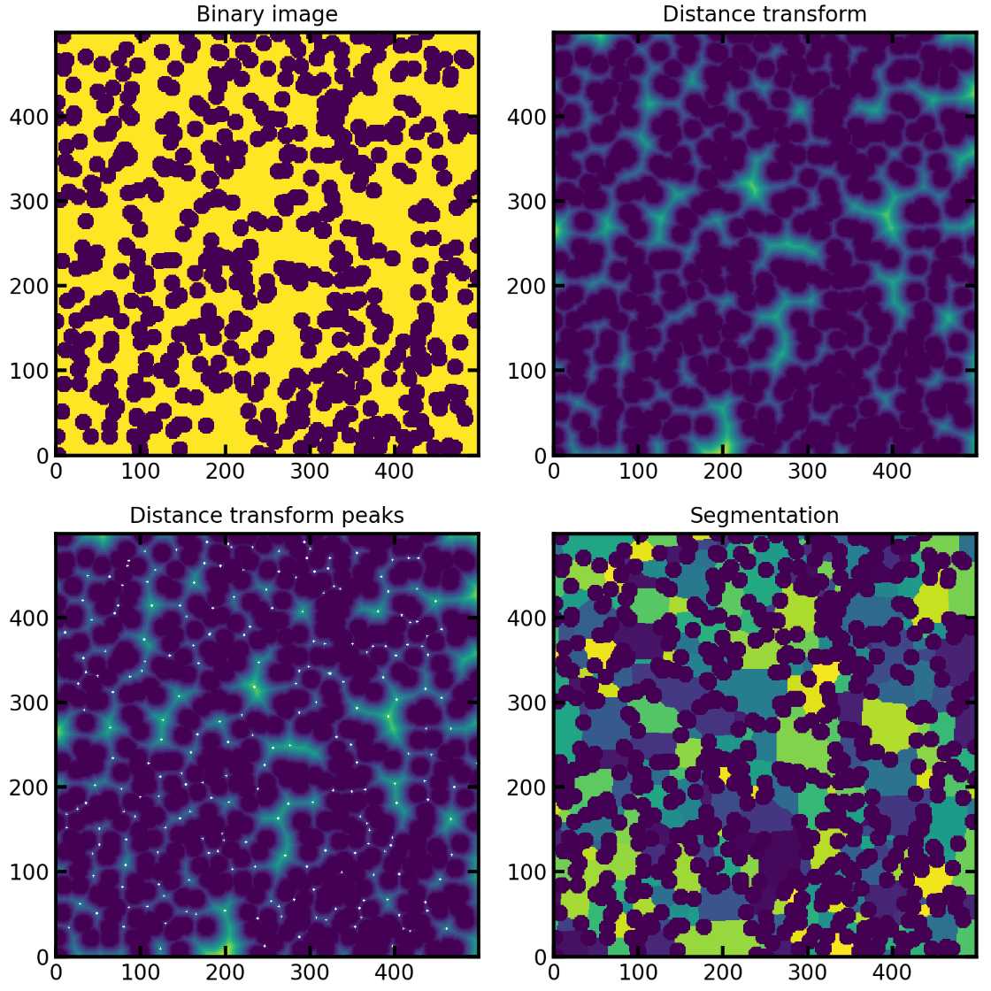
3、提取距离变换和峰值
sigma = 0.4
dt = spim.distance_transform_edt(input=im)#提取距离变换
dt1 = spim.gaussian_filter(input=dt, sigma=sigma)#应用高斯模糊过滤噪声
peaks = find_peaks(dt=dt)#提取峰值

print('Initial number of peaks: ', spim.label(peaks)[1])
peaks = trim_saddle_points(peaks=peaks, dt=dt1)
print('Peaks after trimming saddle points: ', spim.label(peaks)[1])
peaks = trim_nearby_peaks(peaks=peaks, dt=dt)
peaks, N = spim.label(peaks)
print('Peaks after trimming nearby peaks: ', N)
'''
Initial number of peaks:  1539
Peaks after trimming saddle points:  683
Peaks after trimming nearby peaks:  519
'''
def distance_transform_edt(input, sampling=None, return_distances=True,
                           return_indices=False, distances=None, indices=None):
    """
    Exact Euclidean distance transform.

    This function calculates the distance transform of the `input`, by
    replacing each foreground (non-zero) element, with its
    shortest distance to the background (any zero-valued element).

    In addition to the distance transform, the feature transform can
    be calculated. In this case the index of the closest background
    element to each foreground element is returned in a separate array.

    Parameters
    ----------
    input : array_like
        Input data to transform. Can be any type but will be converted
        into binary: 1 wherever input equates to True, 0 elsewhere.
    sampling : float, or sequence of float, optional
        Spacing of elements along each dimension. If a sequence, must be of
        length equal to the input rank; if a single number, this is used for
        all axes. If not specified, a grid spacing of unity is implied.
    return_distances : bool, optional
        Whether to calculate the distance transform.
        Default is True.
    return_indices : bool, optional
        Whether to calculate the feature transform.
        Default is False.
    distances : float64 ndarray, optional
        An output array to store the calculated distance transform, instead of
        returning it.
        `return_distances` must be True.
        It must be the same shape as `input`.
    indices : int32 ndarray, optional
        An output array to store the calculated feature transform, instead of
        returning it.
        `return_indicies` must be True.
        Its shape must be `(input.ndim,) + input.shape`.

    Returns
    -------
    distances : float64 ndarray, optional
        The calculated distance transform. Returned only when
        `return_distances` is True and `distances` is not supplied.
        It will have the same shape as the input array.
    indices : int32 ndarray, optional
        The calculated feature transform. It has an input-shaped array for each
        dimension of the input. See example below.
        Returned only when `return_indices` is True and `indices` is not
        supplied.

    Notes
    -----
    The Euclidean distance transform gives values of the Euclidean
    distance::

                    n
      y_i = sqrt(sum (x[i]-b[i])**2)
                    i

    where b[i] is the background point (value 0) with the smallest
    Euclidean distance to input points x[i], and n is the
    number of dimensions.

    Examples
    --------
    >>> from scipy import ndimage
    >>> import numpy as np
    >>> a = np.array(([0,1,1,1,1],
    ...               [0,0,1,1,1],
    ...               [0,1,1,1,1],
    ...               [0,1,1,1,0],
    ...               [0,1,1,0,0]))
    >>> ndimage.distance_transform_edt(a)
    array([[ 0.    ,  1.    ,  1.4142,  2.2361,  3.    ],
           [ 0.    ,  0.    ,  1.    ,  2.    ,  2.    ],
           [ 0.    ,  1.    ,  1.4142,  1.4142,  1.    ],
           [ 0.    ,  1.    ,  1.4142,  1.    ,  0.    ],
           [ 0.    ,  1.    ,  1.    ,  0.    ,  0.    ]])

    With a sampling of 2 units along x, 1 along y:

    >>> ndimage.distance_transform_edt(a, sampling=[2,1])
    array([[ 0.    ,  1.    ,  2.    ,  2.8284,  3.6056],
           [ 0.    ,  0.    ,  1.    ,  2.    ,  3.    ],
           [ 0.    ,  1.    ,  2.    ,  2.2361,  2.    ],
           [ 0.    ,  1.    ,  2.    ,  1.    ,  0.    ],
           [ 0.    ,  1.    ,  1.    ,  0.    ,  0.    ]])

    Asking for indices as well:

    >>> edt, inds = ndimage.distance_transform_edt(a, return_indices=True)
    >>> inds
    array([[[0, 0, 1, 1, 3],
            [1, 1, 1, 1, 3],
            [2, 2, 1, 3, 3],
            [3, 3, 4, 4, 3],
            [4, 4, 4, 4, 4]],
           [[0, 0, 1, 1, 4],
            [0, 1, 1, 1, 4],
            [0, 0, 1, 4, 4],
            [0, 0, 3, 3, 4],
            [0, 0, 3, 3, 4]]])

    With arrays provided for inplace outputs:

    >>> indices = np.zeros(((np.ndim(a),) + a.shape), dtype=np.int32)
    >>> ndimage.distance_transform_edt(a, return_indices=True, indices=indices)
    array([[ 0.    ,  1.    ,  1.4142,  2.2361,  3.    ],
           [ 0.    ,  0.    ,  1.    ,  2.    ,  2.    ],
           [ 0.    ,  1.    ,  1.4142,  1.4142,  1.    ],
           [ 0.    ,  1.    ,  1.4142,  1.    ,  0.    ],
           [ 0.    ,  1.    ,  1.    ,  0.    ,  0.    ]])
    >>> indices
    array([[[0, 0, 1, 1, 3],
            [1, 1, 1, 1, 3],
            [2, 2, 1, 3, 3],
            [3, 3, 4, 4, 3],
            [4, 4, 4, 4, 4]],
           [[0, 0, 1, 1, 4],
            [0, 1, 1, 1, 4],
            [0, 0, 1, 4, 4],
            [0, 0, 3, 3, 4],
            [0, 0, 3, 3, 4]]])

    """
#trim_saddle_points()
def trim_saddle_points(peaks, dt, maxiter=20):
    r"""
    Removes peaks that were mistakenly identified because they lied on a
    saddle or ridge in the distance transform that was not actually a true
    local peak.

    Parameters
    ----------
    peaks : ndarray
        A boolean image containing ``True`` values to mark peaks in the
        distance transform (``dt``)
    dt : ndarray
        The distance transform of the pore space for which the peaks
        are sought.
    maxiter : int
        The number of iteration to use when finding saddle points.
        The default value is 20.

    Returns
    -------
    image : ndarray
        An image with fewer peaks than the input image

    References
    ----------
    [1] Gostick, J. "A versatile and efficient network extraction algorithm
    using marker-based watershed segmentation".  Physical Review E. (2017)

    Examples
    --------
    `Click here
    `_
    to view online example.

    """
#trim_nearby_peaks()
def trim_nearby_peaks(peaks, dt, f=1):
    r"""
    Removes peaks that are nearer to another peak than to solid

    Parameters
    ----------
    peaks : ndarray
        A image containing nonzeros values indicating peaks in the distance
        transform (``dt``).  If ``peaks`` is boolean, a boolean is returned;
        if ``peaks`` have already been labelled, then the original labels
        are returned, missing the trimmed peaks.
    dt : ndarray
        The distance transform of the pore space
    f : scalar
        Controls how close peaks must be before they are considered near
        to each other. Sets of peaks are tagged as too near if
        ``d_neighbor < f * d_solid``.

    Returns
    -------
    image : ndarray
        An array the same size and type as ``peaks`` containing a subset of
        the peaks in the original image.

    Notes
    -----
    Each pair of peaks is considered simultaneously, so for a triplet of nearby
    peaks, each pair is considered.  This ensures that only the single peak
    that is furthest from the solid is kept.  No iteration is required.

    References
    ----------
    [1] Gostick, J. "A versatile and efficient network extraction
    algorithm using marker-based watershed segmenation". Physical Review
    E. (2017)

    Examples
    --------
    `Click here
    `_
    to view online example.

    """
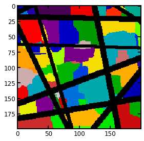
去除杂峰之后就是利用分水岭算法划分孔隙区域
regions = watershed(image=-dt, markers=peaks, mask=dt > 0)
regions = randomize_colors(regions)#赋予不同孔隙区域不同的颜色
fig, ax = plt.subplots()
ax.imshow((regions*im)[:, :, 100], cmap=plt.cm.nipy_spectral);
#watershed()
def watershed(image, markers=None, connectivity=1, offset=None, mask=None,
              compactness=0, watershed_line=False):
    """Find watershed basins in `image` flooded from given `markers`.

    Parameters
    ----------
    image : ndarray (2-D, 3-D, ...)
        Data array where the lowest value points are labeled first.
    markers : int, or ndarray of int, same shape as `image`, optional
        The desired number of markers, or an array marking the basins with the
        values to be assigned in the label matrix. Zero means not a marker. If
        ``None`` (no markers given), the local minima of the image are used as
        markers.
    connectivity : ndarray, optional
        An array with the same number of dimensions as `image` whose
        non-zero elements indicate neighbors for connection.
        Following the scipy convention, default is a one-connected array of
        the dimension of the image.
    offset : array_like of shape image.ndim, optional
        offset of the connectivity (one offset per dimension)
    mask : ndarray of bools or 0s and 1s, optional
        Array of same shape as `image`. Only points at which mask == True
        will be labeled.
    compactness : float, optional
        Use compact watershed [3]_ with given compactness parameter.
        Higher values result in more regularly-shaped watershed basins.
    watershed_line : bool, optional
        If watershed_line is True, a one-pixel wide line separates the regions
        obtained by the watershed algorithm. The line has the label 0.

    Returns
    -------
    out : ndarray
        A labeled matrix of the same type and shape as markers

    See Also
    --------
    skimage.segmentation.random_walker : random walker segmentation
        A segmentation algorithm based on anisotropic diffusion, usually
        slower than the watershed but with good results on noisy data and
        boundaries with holes.

    Notes
    -----
    This function implements a watershed algorithm [1]_ [2]_ that apportions
    pixels into marked basins. The algorithm uses a priority queue to hold
    the pixels with the metric for the priority queue being pixel value, then
    the time of entry into the queue - this settles ties in favor of the
    closest marker.

    Some ideas taken from
    Soille, "Automated Basin Delineation from Digital Elevation Models Using
    Mathematical Morphology", Signal Processing 20 (1990) 171-182

    The most important insight in the paper is that entry time onto the queue
    solves two problems: a pixel should be assigned to the neighbor with the
    largest gradient or, if there is no gradient, pixels on a plateau should
    be split between markers on opposite sides.

    This implementation converts all arguments to specific, lowest common
    denominator types, then passes these to a C algorithm.

    Markers can be determined manually, or automatically using for example
    the local minima of the gradient of the image, or the local maxima of the
    distance function to the background for separating overlapping objects
    (see example).

    References
    ----------
    .. [1] https://en.wikipedia.org/wiki/Watershed_%28image_processing%29

    .. [2] http://cmm.ensmp.fr/~beucher/wtshed.html

    .. [3] Peer Neubert & Peter Protzel (2014). Compact Watershed and
           Preemptive SLIC: On Improving Trade-offs of Superpixel Segmentation
           Algorithms. ICPR 2014, pp 996-1001. :DOI:`10.1109/ICPR.2014.181`
           https://www.tu-chemnitz.de/etit/proaut/publications/cws_pSLIC_ICPR.pdf

    Examples
    --------
    The watershed algorithm is useful to separate overlapping objects.

    We first generate an initial image with two overlapping circles:

    >>> x, y = np.indices((80, 80))
    >>> x1, y1, x2, y2 = 28, 28, 44, 52
    >>> r1, r2 = 16, 20
    >>> mask_circle1 = (x - x1)**2 + (y - y1)**2 >> mask_circle2 = (x - x2)**2 + (y - y2)**2 >> image = np.logical_or(mask_circle1, mask_circle2)

    Next, we want to separate the two circles. We generate markers at the
    maxima of the distance to the background:

    >>> from scipy import ndimage as ndi
    >>> distance = ndi.distance_transform_edt(image)
    >>> from skimage.feature import peak_local_max
    >>> max_coords = peak_local_max(distance, labels=image,
    ...                             footprint=np.ones((3, 3)))
    >>> local_maxima = np.zeros_like(image, dtype=bool)
    >>> local_maxima[tuple(max_coords.T)] = True
    >>> markers = ndi.label(local_maxima)[0]

    Finally, we run the watershed on the image and markers:

    >>> labels = watershed(-distance, markers, mask=image)

    The algorithm works also for 3-D images, and can be used for example to
    separate overlapping spheres.
    """
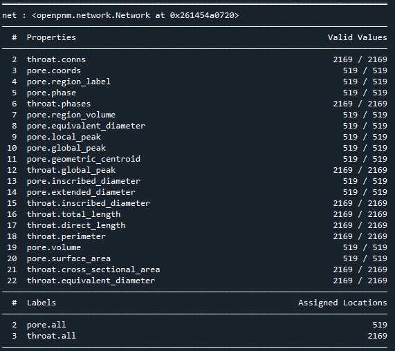
最后提取孔隙网络,在PoreSpy中包含可以将此分区图像传递给网络提取函数,该函数分析图像并返回包含网络数值属性的 Python 字典
net = ps.networks.regions_to_network(regions*im, voxel_size=1)
pn = op.io.network_from_porespy(net)
print(pn)
ax = op.visualization.plot_coordinates(pn)
ax = op.visualization.plot_connections(pn, ax=ax)
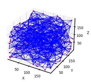
PoreSpy提取的孔隙网络可以直接导入OpenPNM进行渗透率计算,但是通过对比可以发现两者网络模型的相关参数有些许差异,而且与常用的最大球提取法不同,PoreSpy采用SNOW算法提取网络模型,而PoreSpy内置函数里只能计算菲克扩散的扩散系数,没有计算渗透系数的功能,所以具体能否用PoreSpy导出的网络计算渗透率还存疑
Comments NOTHING