1.Intro
To start with, let's first look at the classcial Navier-Stokes Equation
$\frac{\partial \vec{v} }{\partial t} +(\vec{v}\cdot \nabla )\vec{v}=-\nabla p +\nu \nabla ^{2}\vec{v} $
$\vec{v}$ : velocity field, having different values in space
$\frac{\partial \vec{v} }{\partial t}$ : unsteady term, indicating the change of velocity with time
$(\vec{v}\cdot \nabla )\vec{v}$ : convective acceleration term, non-linear
$\bigtriangledown p$ : gradient of thermodynamic pressure
$\nu \nabla ^{2}\vec{v}$ : represent the viscous diffusion
Assumption:
- Newtonian fluid: stress and strain rate are linearly related
- The density $\rho$ is constant:no compressibility effect
When we assume that $\nu =0$, the 2nd order in Navier-Stokes Equation turns to 0(inviscid fluid), which turns Navier-Stokes Equation into the Euler Equation.
In CFD, any assumption will result in errors, it's usual that there exist discrepancies between a CFD solution and an experiment(mathematical model and physical model)
Euler Equation:
$\frac{\partial \vec{v} }{\partial t} +(\vec{v}\cdot \nabla )\vec{v}=-\nabla p $
The acceration has two components, one component represents how velocity changes with respect to time, the other one represents how the velocity changes because a particle fluid moves from one place to another place(conviction).
1.1 The basic ingredients of CFD
1.1.1 different mathematical models
The characteristics of these models/equations:
- have a set of partial differential equations or intergal differential equations
- associate with boundary conditions
- use target applications to simplify the model, like incompressible, inviscid, turbulent, 2d or 3d
1.1.2 choose discretization method
To choose discretization method invovles two aspects:
- discretize geometry: the basic geometry is called grid/mesh(grid gives the vessel of the solution)
-
discretize the model: transform the continum mathematical operators into arithmatic operators on the grid values
The discretization method is for approximation the PDEs by a system of algebraic equations, usually we have different discretization methods, as followed:
- finite difference(FD)
- finite volume(FV)
- finite elements(FE)
- spectral methods
- boundary dement method(BEM)
- particle methods
1.1.3 analyze the numerical scheme
We use these schemes to obtain the grid point values of all the flow variables, usually they are
- time dependent situation
- steady situation
All the numercial schemes must satisfy certain conditions to be accepted:
- consistancy
- stability
-
convegence
Also we must analyze accuracies of all the schemes.
1.1.4 solve
1.1.5 post-processing, visualizaiton
## 2. The derivation of the differential form for the fluid equations
2.1.1 Conservation of Mass(a.k.a. Continuity)
- for a system:
$\frac{\mathrm{d} M_{sys} }{\mathrm{d} t} =0$ - for a control voulme:
$\frac{\partial \int\limits_{c.v.}^{}\rho \mathrm{d}v }{\partial t} + \int\limits_{c.s.}^{}\rho \vec{v}\cdot \hat{n} \mathrm{d}tA=0 $- $\frac{\partial \int\limits_{c.v.}^{}\rho \mathrm{d}v }{\partial t}$ rate of change of mass in control volume
- $\int\limits_{c.s.}^{}\rho \vec{v}\cdot \hat{n} \mathrm{d}tA$ net rate of mass flow across the control surface
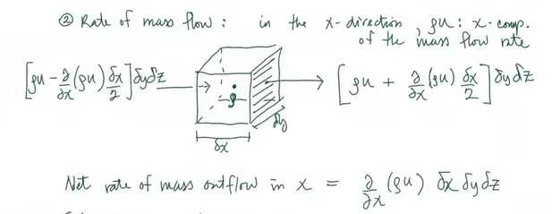
Differential Form of volume- consider a small element $\partial x\partial y\partial z$
so we get new forms of seperate term above:
$\frac{\partial \int\limits_{c.v.}^{}\rho \partial x \partial y \partial z }{\partial x}$
Rate of mass flow:
mass flow is in the x direction, and in the center of this cube, the density is equal to $\rho$, so the x-component quantity is equal to $\rho u$, and we do a Talyor expansion, then the $\rho u$ becomes $(\rho u +\frac{\partial (\rho u)}{\partial x} \cdot \frac{\delta x}{2})\mathrm{d}y \mathrm{d}z $
Net rate of mass outflow in x:$\frac{\partial (\rho u)}{\partial x} \cdot \mathrm{d}x\mathrm{d}y\mathrm{d}z$
similarly,
in y: $\frac{\partial (\rho u)}{\partial y} \cdot \mathrm{d}x\mathrm{d}y\mathrm{d}z$
in z: $\frac{\partial (\rho u)}{\partial z} \cdot \mathrm{d}x\mathrm{d}y\mathrm{d}z$
then we have differential form of conservation of mass:
$\frac{\partial\rho}{\partial t}+\frac{\partial (\rho u)}{\partial x}+\frac{\partial (\rho u)}{\partial y} +\frac{\partial (\rho u)}{\partial z}=0 $
vector notation(continuity equation): $\frac{\partial\rho}{\partial t}+\nabla \rho\cdot \vec{v} =0$
2.1.2 Conservation of the Momentum
2.1.2.1 Conservation of Momentum
- for a system:
$\vec{F} =\frac{\mathrm{d} \int\limits_{sys}^{} \vec{v}\mathrm{d}m }{\mathrm{d} x}$ - for a control volume:
$\sum \vec{F_{c.v.} } =\frac{\partial \int\limits_{c.v.}^{} \vec{v} \rho dv}{\partial t}+\int\limits_{c.s.}^{}\vec{v}\rho \vec{v} \cdot \hat{n} \mathrm{d}A$- ${\int\limits_{c.v.}^{} \vec{v} \rho dv}$: element of mass
- $\int\limits_{c.s.}^{}\vec{v}\rho \vec{v} \cdot \hat{n} \mathrm{d}A$: flux term, represents the flux of the momentum
2.1.2.2 Infinitesimal fluid mass $\mathrm{d}m$
$\mathrm{d}\vec{F} =\frac{\mathrm{d} (\vec{v}\mathrm{d}m) }{\mathrm{d}t} = \mathrm{d}m \frac{\mathrm{d} \vec{v}}{\mathrm{d} t}=\mathrm{d}m\cdot \vec{a}$
2.1.2.3 Types of forces and stresses:
- Forces:
- body forces: weight $\mathrm{d}\vec{F} = \mathrm{d}m\cdot \vec{g}$
- surface forces:
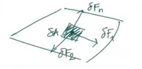
- normal: $\mathrm{d}F_n$
- tangential: $\mathrm{d}F_1,\mathrm{d}F_2$
有两种力,一种面内,一种面外,两种力两两正交
- Stresses:
- Normal Stress: $\sigma n=\lim{\mathrm{d}A \to 0} \frac{\mathrm{d} \vec{F_n}}{\mathrm{d} A} $
- Shearing Stresses:
- $\tau 1=\lim{\mathrm{d}A \to 0} \frac{\mathrm{d} \vec{F_1}}{\mathrm{d} A} $
- $\tau 2=\lim{\mathrm{d}A \to 0} \frac{\mathrm{d} \vec{F_2}}{\mathrm{d} A} $
With reference to a coordinate system:
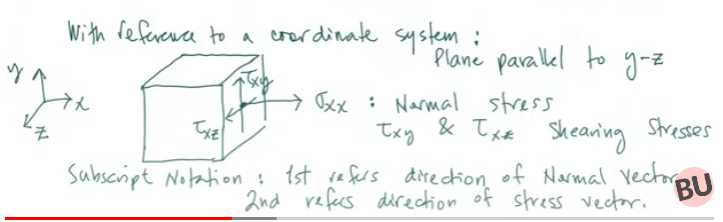
图中为单元体中应力的方向
应力方向确定:
正应力:拉为正,压为负
剪应力:正面正向,负面负向为正,其余为负
Surface forces in terms of stresses:
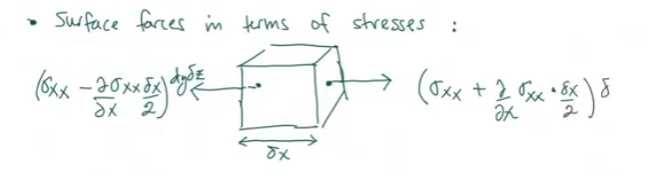
In X direction:
A pair of normal stresses on the surface:
$(\sigma _{xx}-\frac{\partial \sigma _{xx}}{\partial x} \frac{\mathrm{d}x}{2} )\mathrm{d}y \mathrm{d}z $
$(\sigma _{xx}+\frac{\partial \sigma _{xx}}{\partial x} \frac{\mathrm{d}x}{2} )\mathrm{d}y \mathrm{d}z $
A pair of shear stresses on the surface:
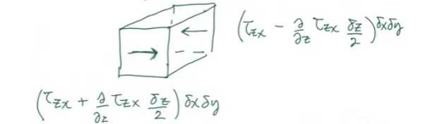
$(\tau _{zx}-\frac{\partial \tau _{zx}}{\partial z}\frac{\mathrm{d}z }{2} )\mathrm{d}x \mathrm{d}y $
$(\tau _{zx}+\frac{\partial \tau _{zx}}{\partial z}\frac{\mathrm{d}z }{2} )\mathrm{d}x \mathrm{d}y $
A pair of shear stresses on the surface:
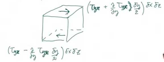
$(\tau _{yx}-\frac{\partial \tau _{yx}}{\partial y}\frac{\mathrm{d}z }{2} )\mathrm{d}x \mathrm{d}z$
$(\tau _{yx}+\frac{\partial \tau _{yx}}{\partial y}\frac{\mathrm{d}z }{2} )\mathrm{d}x \mathrm{d}z $
X direction:
$\mathrm{d}F_{sx} =(\frac{\partial{} \sigma {xx}}{\partial{x} }+\frac{\partial \tau{yx}}{\partial y}+\frac{\partial \tau_{zx}}{\partial z})\mathrm{d}x \mathrm{d}y \mathrm{d}z $
Y direction:
$\mathrm{d}F_{sy} =(\frac{\partial \tau_{xy}}{\partial x}+\frac{\partial{} \sigma {yy}}{\partial{y} }+\frac{\partial \tau{zy}}{\partial z})\mathrm{d}x \mathrm{d}y \mathrm{d}z $
Z direction:
$\mathrm{d}F_{sz} =(\frac{\partial \tau_{xz}}{\partial x}+\frac{\partial \tau_{yz}}{\partial y}+\frac{\partial{} \sigma _{zz}}{\partial{z} })\mathrm{d}x \mathrm{d}y \mathrm{d}z $
We know that $\mathrm{d}\vec{F} =\mathrm{d}m\cdot \vec{a}$ and $\mathrm{d}m=\rho\mathrm{d}x \mathrm{d}y\mathrm{d}z$
Then we have:
$\rho g_{x}+\frac{\partial{} \sigma {xx}}{\partial{x} }+\frac{\partial \tau{yx}}{\partial y}+\frac{\partial \tau_{zx}}{\partial z}=\rho (\frac{\partial u}{\partial t}+u\frac{\partial u}{\partial x}+v\frac{\partial u}{\partial y}+w\frac{\partial u}{\partial z} ) $
similarly in other directions:
$\rho g_{x}+\frac{\partial \tau_{xy}}{\partial x}+\frac{\partial{} \sigma {yy}}{\partial{y} }+\frac{\partial \tau{zy}}{\partial z}=\rho (\frac{\partial u}{\partial t}+u\frac{\partial v}{\partial x}+v\frac{\partial v}{\partial y}+w\frac{\partial v}{\partial z} ) $
$\rho g_{x}+\frac{\partial \tau_{xz}}{\partial x}+\frac{\partial \tau_{yz}}{\partial y}+\frac{\partial{} \sigma _{zz}}{\partial{z} }=\rho (\frac{\partial u}{\partial t}+u\frac{\partial w}{\partial x}+v\frac{\partial w}{\partial y}+w\frac{\partial w}{\partial z} ) $
Now we have 3 equations above and continuity equation, there are 4 equations. In these equations, we don't know the three components of velocity $u,v,w$ and all the stresses. To solve these equations ,we need to make some assumptions.
Assumption:
* For inviscid flow: no shearing stresses and all the normal stresses are equal to $-p$.
Then the Euler Equation is equal to:
$\rho g_{x}-\frac{\partial{} p}{\partial{x} }=\rho (\frac{\partial u}{\partial t}+u\frac{\partial u}{\partial x}+v\frac{\partial u}{\partial y}+w\frac{\partial u}{\partial z} ) $
Vector Notation:
$\rho \vec{g}-\bigtriangledown p=\rho (\frac{\partial \vec{v}}{\partial t}+(\vec{v}\cdot \bigtriangledown)\vec{v})$
3. The Navier-Stokes Equations
Newtonian Fluid
- Linear relationship between stresses
- Linear relatoinship between rates of deformation
Normal stresses:
$\sigma_{xx}=-p+2\mu\frac{\partial u}{\partial x}$
$\sigma_{yy}=-p+2\mu\frac{\partial v}{\partial y}$
$\sigma_{zz}=-p+2\mu\frac{\partial w}{\partial z}$
$\sigma_{xx}+\sigma_{yy}+\sigma_{zz}=-3p$
Shear stresses:
$\tau_{xy}=\tau_{yx}=\mu(\frac{\partial u}{\partial y}+\frac{\partial v}{\partial x})$
$\tau_{yz}=\tau_{zy}=\mu(\frac{\partial v}{\partial z}+\frac{\partial w}{\partial y})$
$\tau_{zx}=\tau_{xz}=\mu(\frac{\partial w}{\partial x}+\frac{\partial u}{\partial z})$
Stress terms, x-direction momentum equ:
$\frac{\partial \sigma_{xx}}{\partial x}+\frac{\partial \tau_{yx}}{\partial y}+\frac{\partial \tau_{zx}}{\partial z}$
4. Finite Difference Method(FDM)
原文出自 微分方程数值求解——有限差分法,作者:科研民工,作者写的非常好,此处将其搬运过来。
3.1 引言
有限差分法(Finite Difference Method,FDM)是一种求解微分方程数值解的近似方法,其主要原理是对微分方程中的微分项进行直接差分近似,从而将微分方程转化为代数方程组求解。有限差分法的原理简单,粗暴有效,最早由远古数学大神欧拉(L. Euler 1707-1783)提出,他在1768年给出了一维问题的差分格式。1908年,龙格(C. Runge 1856-1927)将差分法扩展到了二维问题【对,就是龙格-库塔法中的那个龙格】。但是在那个年代,将微分方程的求解转化为大量代数方程组的求解无疑是将一个难题转化为另一个难题,因此并未得到大量的应用。随着计算机技术的发展,快速准确地求解庞大的代数方程组成为可能,因此逐渐得到大量的应用。发展至今,有限差分法已成为一个重要的数值求解方法,在工程领域有着广泛的应用背景。本文将从有限差分法的原理、基本差分公式、误差估计等方面进行概述,给出其基本的应用方法,对于一些深入的问题不做讨论。
3.2 FDM方法概述
首先,有限差分法是一种求解微分方程的数值方法,其面对的对象是微分方程,包括常微分方程和偏微分方程。此外,有限差分法需要对微分进行近似,这里的近似采取的是离散近似,使用某一点周围点的函数值近似表示该点的微分。下面将对该方法进行概述。
3.2.1 有限差分法的基本原理
这里我们使用一个简单的例子来简述有限差分法的基本原理,考虑如下常微分方程
$\left{\begin{array}{l}u^{\prime}(x)+c(x) u(x)=f(x), \quad x \in[a, b] \ u(x=a)=d\end{array}\right. \quad (1)$
微分方程与代数方程最大的不同就是其包含微分项,这也是求解微分方程最难处理的地方。有限差分法的基本原理即使用近似方法处理微分方程中的微分项。为了得到微分的近似,我们最容易想到的即导数定义
$u^{\prime}(x)=\lim _{\Delta x \rightarrow 0} \frac{u(x+\Delta x)-u(x)}{\Delta x} \approx \frac{u(x+\Delta x)-u(x)}{\Delta x} \quad (2)$
上式后面的近似表示使用割线斜率近似替代切线斜率,即为步长,如图 1(a)所示。式(2)表明函数在某一点的微分可以由相邻点的函数值近似确定。显然,这里微分近似的精度与步长的选取有关,步长越短则越精确。
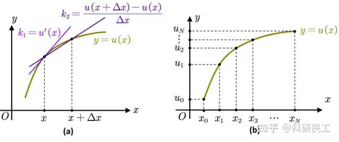
图1. (a)微分的近似表示 (b)一维区间的离散表示
因此,这里首先需要对求解域进行离散,然后分别得到各离散点上的微分近似。对于示例的一维问题,将求解区间等分为$N$个区间,步长为$h$,分别将包含首尾的各结点记为$x_0, x_1, x_2, x_3, \ldots x_N$,对应的函数值为$u_0, u_1, u_2, \ldots, u_N$,这样,就把原问题的求解转化为了各结点函数值$u_i$的求解。式(2)的离散形式表示为
$u_i^{\prime}=\frac{1}{h}\left(u_{i+1}-u_i\right), \quad i=0,1,2, \ldots, N-1 \quad (3)$
将式(3)代入方程(1)可以得到
$\left{\begin{array}{l}\left(u_{i+1}-u_i\right) / h+c\left(x_i\right) u_i=f\left(x_i\right) \u_0=d
\end{array} ; \quad i=1,2, \ldots, N-1\right. \quad (4)$
这里的结点坐标$x_i=a+ih,(i=0,1,2,3,4)$,步长$h=(b-a)/N$均为已知。$c_i=c(x_i), f_i=f(x_i)$,将式(4)合并同类项可以得到如下递推关系
$u_{i+1}=(1-hc_{i})u_{i}+hf_{i}$
$u_{0}=d$
上式共有$N$个方程,包括$N$个未知数$u_0, u_1, u_2, \ldots, u_N$,刚好可以求解得到各结点上的待求函数的值,从而得到原问题在求解域上的近似解。由于该问题中初值已给定,按照各结点依次迭代就可以得到该问题的解。此外,为了给出更一般化的求解方法,可以将(5)写成矩阵的形式,即
$Au=F$
$\left[\begin{array}{cccc}1 & & & \ C_1 & 1 & & \ & \ddots & \ddots & \ & & C_{N-1} & 1\end{array}\right]\left{\begin{array}{c}u_1 \ u_2 \ \vdots \ u_N\end{array}\right}=\left{\begin{array}{c}F_0 \ F_1 \ \vdots \ F_{N-1}\end{array}\right}-\left{\begin{array}{c}C_0 u_0 \ 0 \ \vdots \ 0\end{array}\right}$
其中,$C_i=hc_i-1, F_i=hf_i$,显然矩阵A可逆,因此上述问题的解为$u=A^{-1}F$
3.2.2 微分的近似表示
上一节以一个一维一阶微分方程为例简单描述了有限差分的基本原理,下面我们对其更广泛的使用进行扩展。注意到式(3)中的一阶微分是使用相邻结点的函数值来表示,一般地,假设函数$u(x)$在求解域内连续可导,则由泰勒级数我们可以得到
$u(x+h)=u(x)+h u^{\prime}(x)+\frac{h^2}{2} u^{\prime \prime}(x)+\cdots+\frac{h^k}{k !} u^{(k)}(x)+\dots \quad(9)$
基于泰勒级数并做适当的截断,我们就可以得到各阶微分的近似表达式,或者记做“差分公式”。下面主要对一阶和二阶微分的差分公式进行讨论,更高阶的微分可以同理推导得到。
3.2.2.1 一阶微分
我们将(8)式另写作
$u(x+h)=u(x)+h u^{\prime}(x)+\frac{h^2}{2} u^{\prime \prime}(x)+\frac{h^3}{6} u^{(3)}(x+\xi)+\dots \quad(10)$
这里$\xi \in(0,h)$,对上式变形即可以得到一阶微分的向前差分公式:
$u_F^{\prime}=\frac{u(x+h)-u(x)}{h}-\frac{h}{2}u^{\prime\prime}(x+\xi)\quad(11)$
将(10)式中的$h$用$-h$替代,则可以得到一阶微分的向后差分公式:
$u_F^{\prime}=\frac{u(x)-u(x-h)}{h}+\frac{h}{2}u^{\prime\prime}(x+\xi)\quad(12)$
联立式(11)与(12),则可以得到一阶微分的中心差分公式:
$u_{F}^{\prime}=\frac{u(x+h)-u(x-h)}{2h}-\frac{h^2}{6}u^{\prime\prime\prime}(x+\xi) \quad(13)$
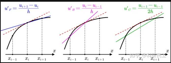
式(11)-(13)是几种常用的一阶微分的差分公式,式(11)-(13)中右边的最后一项即为截断误差。由于这里的误差与步长相关,因此可以看到向前和向后差分公式具有一阶近似精度$O(h)$,而中心差分则具有二阶近似精度$O(h^2)$,三种差分公式的区别如图(3)所示。
Comments NOTHING