2. Probability

For observation of a random phenomenon, the probability of a particular outcome is the proportion of times that outcome would occur in an indefinitely long sequence of like observations, under the same conditions.

• complement 补
• intersection 交 (and)
• union 并 (or)
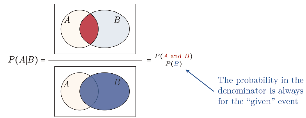
• A probability of event $ A $, given event $ B $ occurred, is called conditional probability. It is denoted by $ P(A \mid B) $.
  

  Placing P(B) in the denominator corresponds to conditioning on (i.e., restricting to) the sample points in B, and it requires P(B)>0. We place P(A B) in the numerator to find the fraction of event $ B $ that is also in event $ A $ (see Figure 2.3).

  

  $$
  P(A \mid B)=\frac{P(A B)}{P(B)}
  $$

• Random variable: For a random phenomenon, a random variable is a function that assigns a numerical value to each point in the sample space. Random variables can be discrete or continuous. We use
  • upper-case letters to represent random variables,
  • with lower-case versions for particular possible values.
• Probability distribution: A probability distribution lists the possible outcomes for a random variable and their probabilities.
  • Probability density function for continuous random variables (pdf)
  • probability mass function for discrete random variable (pmf)
  • Cumulative distribution function (cdf)

  The probability $ P(Y \leq y) $ that a random variable $ Y $ takes value $ \leq y $ is called a cumulative probability. The cumulative distribution function is $ F(y) = P(Y \leq y) $, for all real numbers $ y $.

  By convention, we denote a pdf or pmf by lower-case $ f $ and a c d f by upper-case $ F $.

  $$
  F(y) = P(Y \leq y) = \int_{-\infty}^{y} f(u) d u .
  $$

  Because we obtain the cdf for a continuous random variable by integrating the pdf, we can obtain the pdf from the cdf by differentiating it.

• Expected value (mean, expectation) of a discrete random variable:

• $$
  E(Y)=\sum_{y} y f(y),
  $$

• For a discrete random variable $ Y $ with pmf $ f(y) $ and $ E(Y)=\mu $, the variance is denoted by $ \sigma^{2} $ and defined to be:

• $$
  \sigma^{2}=E(Y-\mu)^{2}=\sum_{y}(y-\mu)^{2} f(y),
  $$

  The variance of a discrete (or continuous) random variable has an alternative formula, resulting from the derivation:

  $$
  \begin{aligned}
  \sigma^{2} & =E(Y-\mu)^{2}=\sum_{y}(y-\mu)^{2} f(y) \\
  & =\sum_{y}\left(y^{2}-2 y \mu+\mu^{2}\right) f(y) \\
  & = \sum_{y} y^{2} f(y)-2 \mu \sum_{y} y f(y)+\mu^{2} \sum_{y} f(y) \\
  & =E\left(Y^{2}\right)-2 \mu E(Y)+\mu^{2} \\
  & =E\left(Y^{2}\right)-\mu^{2}
  \end{aligned}
  $$

  $$
  \operatorname{var}(Y)=\sigma^{2}=E\left(Y^{2}\right)-\mu^{2}
  $$

• The standard deviation of a discrete random variable, denoted by $ \sigma $, is the positive square root of the variance.
• Expected value and variability of a continuous random variable for a continuous random variable $ Y $ with probability density function $ f(y) $,

• $$
  E(Y)=\mu=\int_{y} y f(y) d y , \\
  \text { variance } \sigma^{2}=E(Y-\mu)^{2}=\int_{y}(y-\mu)^{2} f(y) d y,
  $$

  and the standard deviation \sigma is the positive square root of the variance.

Bayes’ theorem

For any two events $ A $ and $ B $ in a sample space with $ P(A)>0 $,

$$
P(B \mid A)=\frac{P(A \mid B) P(B)}{P(A \mid B) P(B)+P\left(A \mid B^{c}\right) P\left(B^{c}\right)}
$$

Generally, for two events $ A $ and $ B $, the multiplicative law of probability states that:

$$
P(A B)=P(A \mid B) P(B)=P(B \mid A) P(A) .
$$

Sometimes $ A $ and $ B $ are independent events, in the sense that $ P(A \mid B)=P(A) $, that is, whether $ A $ occurs does not depend on whether $ B $ occurs. In that case, the previous rule simplifies:

$$
P(A B)=P(A) P(B) .
$$