Session 9 pumapy: Image Import and Manipulation
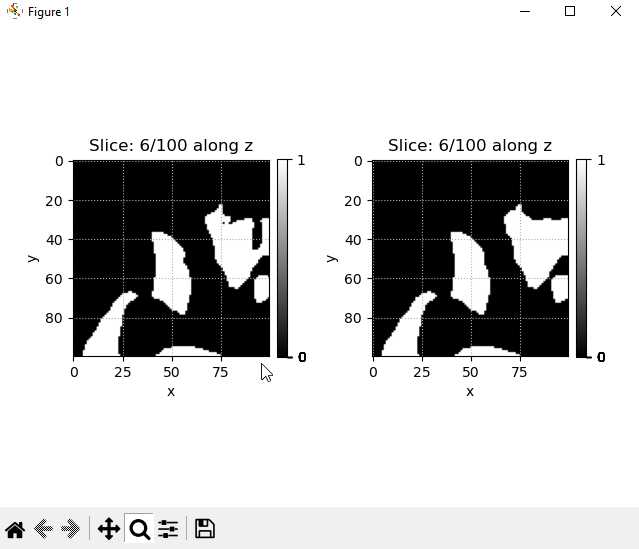
The following snippet shows how to use the filter closing and dialation operations to remove small pores and fill small throats in a 3D image in PuMA py.
import pumapy as puma
import pyvista as pv

ws = puma.import_3Dtiff(puma.path_to_example_file("100_fiberform.tif"), 1.3e-6)
ws_closing = ws.copy()

# erode and dilate the workspace
puma.filter_closing(ws_closing, cutoff=(90, 255), size=3)

ws_binary = ws.copy()
ws_binary.binarize_range((90, 255))

puma.compare_slices(ws_binary, ws_closing, "z", index=1)

p = pv.Plotter(shape=(1, 2))
ws.voxel_length = 1  # the voxel_length is converted to 1 for plotting the workspace together with the velocity
p.subplot(0, 0)
p.add_text("Closing")
By executing the code, one will be able to view the following figure that compares the image slices before and after filtering. The mouse wheel (middle button) can be used to scroll through the slices.
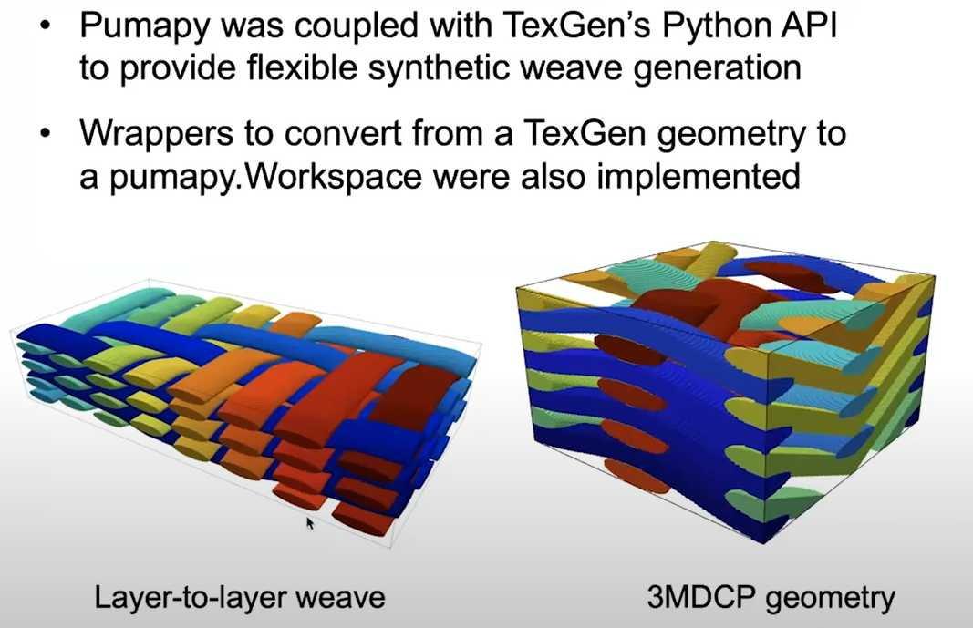
Session 10 Weave Generation via TexGen integration
Linux OS
from TexGen.Core import *
NumBinderLayers = 2
NumXYarns = 3
NumYYarns = 4
XSpacing = 1.0
YSpacing = 1.0
XHeight = 0.2
YHeight = 0.2
weave = CTextileLayerToLayer(NumXYarns, NumYYarns, XSpacing, YSpacing, XHeight, YHeight, NumBinderLayers)
#set number of binder / warp yarns
NumBinderYarns = 2
NumWarpYarns = NumXYarns - NumBinderYarns
weave.SetWarpRatio(NumWarpYarns)
weave.SetBinderRatio(NumBinderYarns)
#setup layers: 3 warp, 4 weft
weave.SetupLayers( 3, 4, NumBinderLayers)
#set yarn dimensions: widths / heights
weave.SetYYarnWidths(0.8)
weave.SetYYarnWidths(0.8)
weave.SetBinderYarnWidths(0.4)
weave.SetBinderYarnHeights(0.1)
#define offsets for the two binder yarns
P = [[0, 1, 3, 0],[3, 0, 0, 3]]
#assign the z-positions to the binder yarns
for y in range(NumWarpYarns,NumXYarns): #loop through number of binder yarns
offset = 0
for x in range(NumYYarns): #loop through the node positions
weave.SetBinderPosition(x, y, P[y-NumWarpYarns][offset])
offset += 1
weave.AssignDefaultDomain()
domain = weave.GetDefaultDomain()
"""
Note that the code above is actually calling TexGen to generate the textile structure. Therefore it can be run independently (of puma) in TexGen as well.
"""
export_path = "out" # CHANGE THIS PATH
if not os.path.exists(export_path):
os.makedirs(export_path)
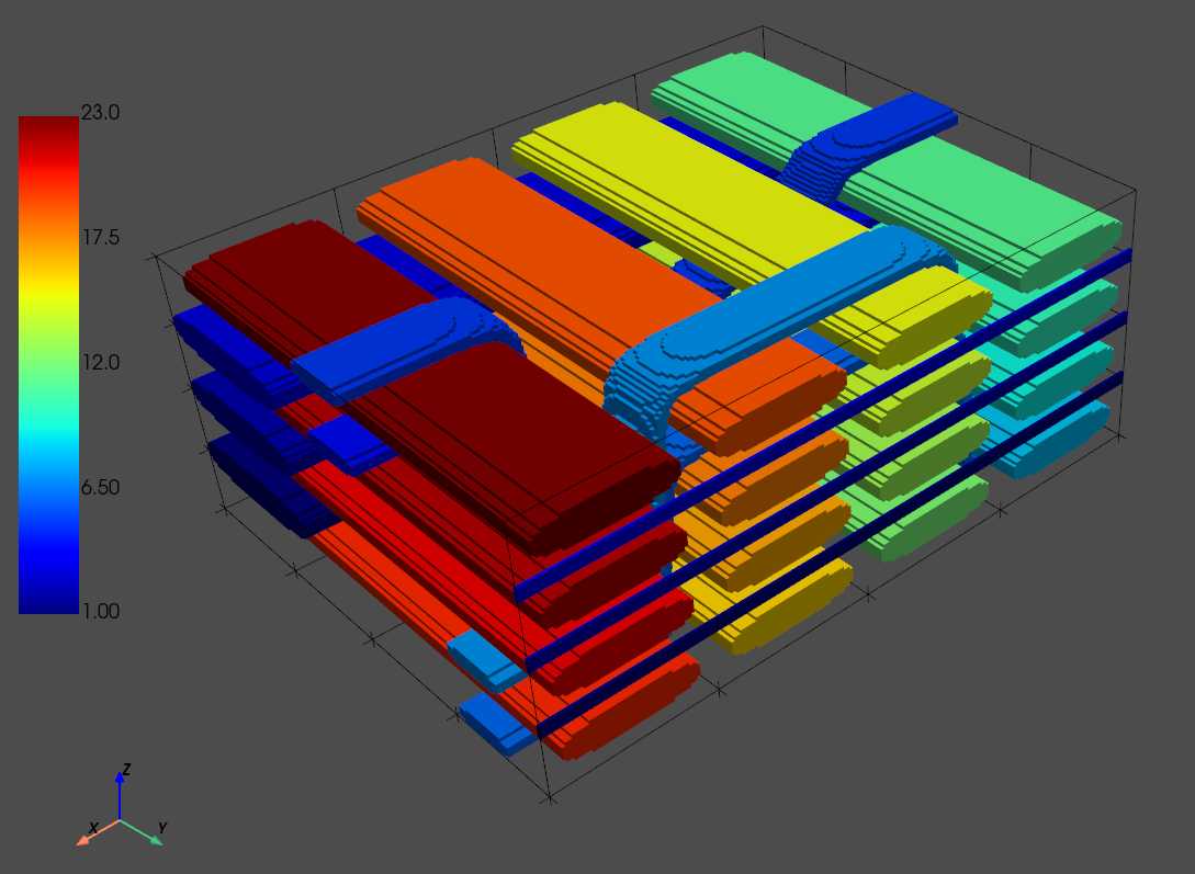
puma.export_weave_vtu(os.path.join(export_path, "weavetest"), weave, domain, 200)
ws = puma.import_weave_vtu(os.path.join(export_path, "weavetest_200"))
puma.render_volume(ws, cutoff=(1, ws.matrix.max()), solid_color=None, notebook=notebook, cmap='jet')
Windows
On windows one can use the GUI of TexGen to generate a voxel model and save it as a .vtu file. Then the following code in PuMApy can take the file:
path = os.path.join(export_path, "weavetest_200")
ws = puma.import_weave_vtu(path)
puma.render_volume(ws, cutoff=(1, ws.matrix.max()), solid_color=None, notebook=notebook, cmap='jet')
More microstructures
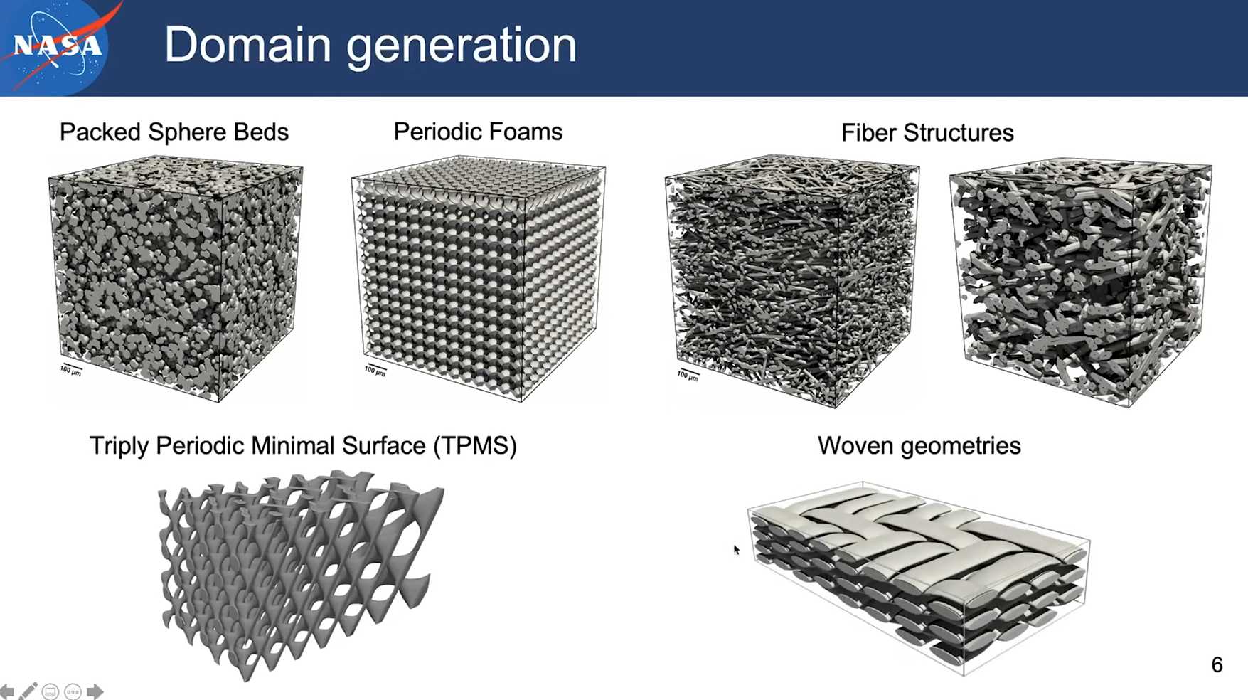
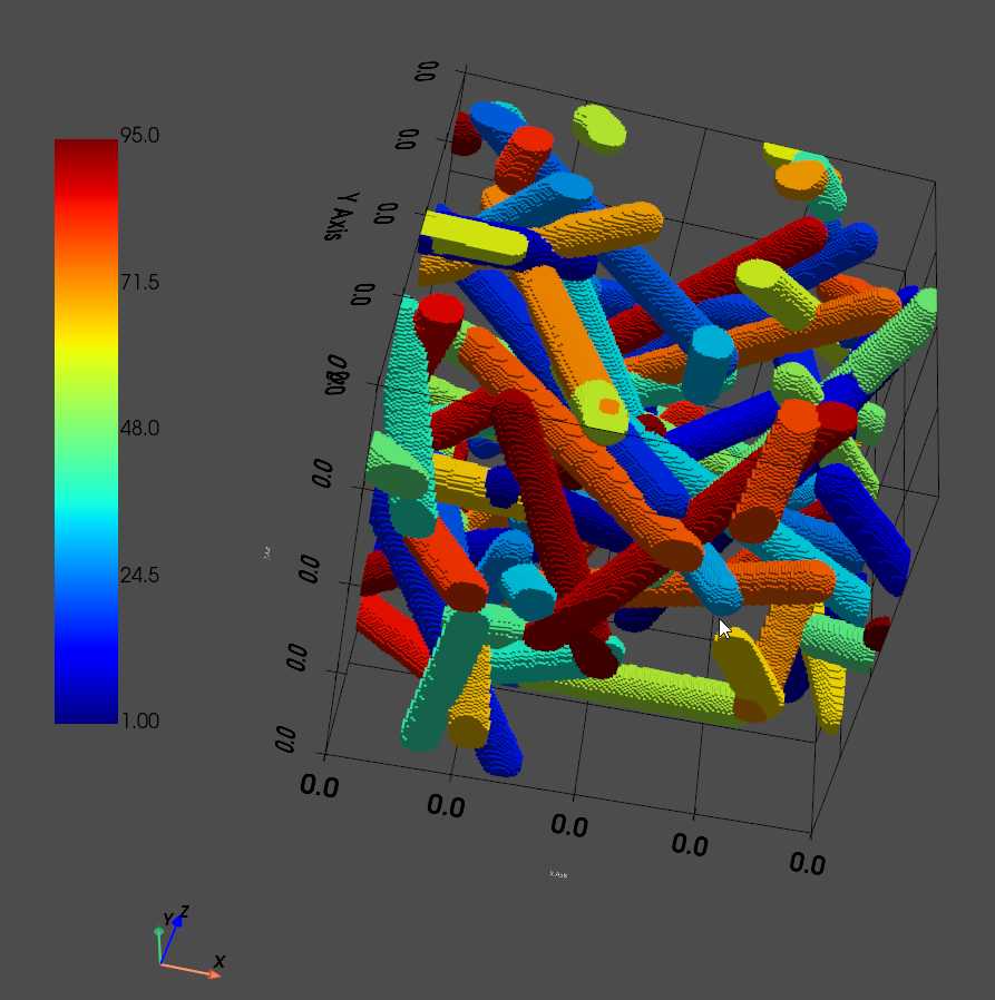
1. Random fibers
import pumapy as puma
import os

notebook = False  # when running locally, actually open pyvista window

size = (200, 200, 200)  # size of the domain, in voxels.
radius = 8  # radius of the fibers to be generated, in voxels
nFibers = None  # Can specify either the number of fibers or the porosity
porosity = 0.8  # porosity of the overall structure
length = 200  # Length of the fibers to be generated
max_iter = 3  # optional (default=3), iterations to refine the porosity
allow_intersect = True  # optional (default=True), allow intersection betweem the fibers: if equal to False, the function runs considerably more slowly because
# randomly proposed fibers are rejected if they intersect any other fiber - use with relatively high porosity for reasonable runtimes
segmented = True  # assign unique IDs to each fiber (if set to False, range will be from 0-255)

ws_fibers_isotropic = puma.generate_random_fibers_isotropic(size, radius, nFibers, porosity, length, allow_intersect=allow_intersect, segmented=segmented)

puma.render_volume(ws_fibers_isotropic, (1, ws_fibers_isotropic.max()), solid_color=None, cmap='jet', style='surface', notebook=notebook)
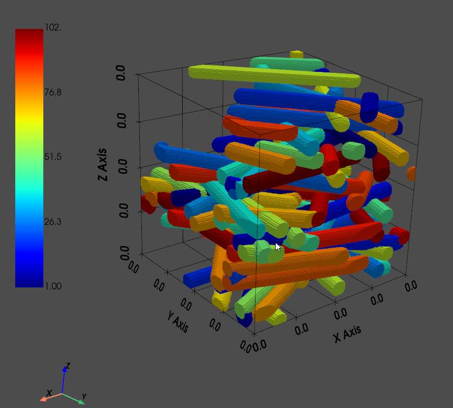
2. Transverse isotropic fibers
direction = 'z'  # Direction orthogonal to the fibers. For example, 'z' means fibers are oriented in the XY plane.
variation = 0  # Variability for the angle, relative to the XY plane. Should be between 0 and 90.

ws_fibers_trans_iso = puma.generate_random_fibers_transverseisotropic(size, radius, nFibers, porosity, direction, variation, length, allow_intersect=allow_intersect, segmented=segmented)
puma.render_volume(ws_fibers_trans_iso, cutoff=(1, ws_fibers_trans_iso.max()), solid_color=None, cmap='jet', notebook=notebook)
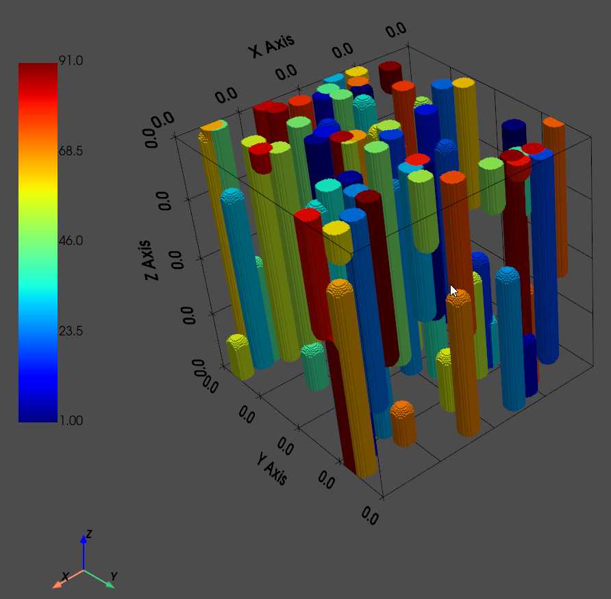
3. Aligned 1D fiber structures
direction = 'z'  # Direction of the 1D fibers.
ws_fibers_1D = puma.generate_random_fibers_1D(size, radius, nFibers, porosity, direction, length, allow_intersect=allow_intersect, segmented=segmented)
puma.render_volume(ws_fibers_1D, cutoff=(1, ws_fibers_1D.max()), solid_color=None, cmap='jet', notebook=notebook)
To plot the result slice by slice, one can use:
puma.plot_slices(ws_fibers_isotropic)
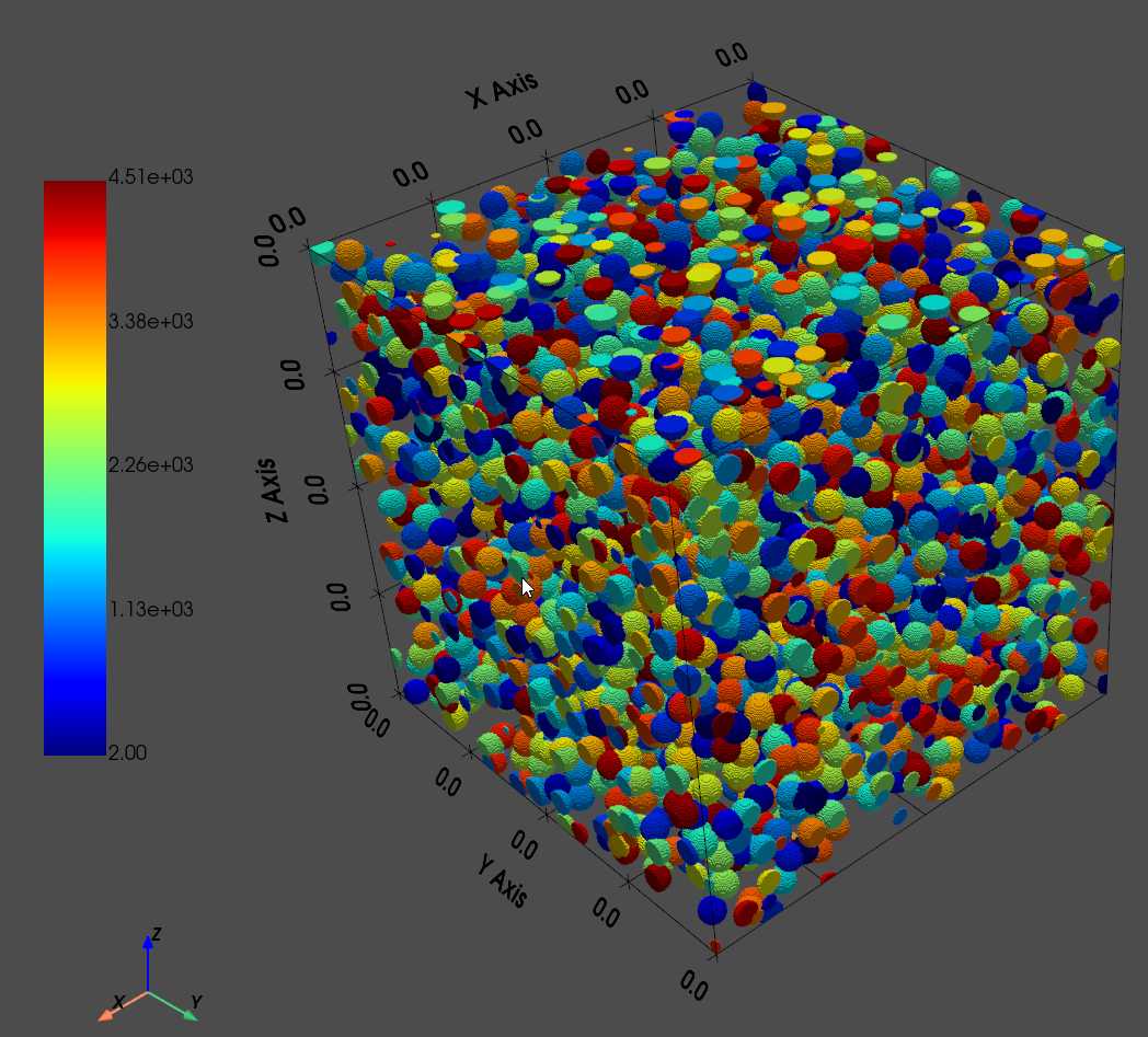
4. Generating Random Sphere Structures
size = (400, 400, 400)  # size of the domain, in voxels.
diameter = 20  # diameter of the spheres to be generated, in voxels
porosity = 0.8  # porosity of the overall structure
allow_intersections = True # flag on whether to allow intersections between spheres.
segmented = True  # assign unique IDs to each sphere (if set to False, range will be from 0-255)
# Note: If allow_intersections is set to false, it will be significantly slower to generate,
#       and will usually require a fairly high porosity value to be generated

ws_spheres = puma.generate_random_spheres(size, diameter, porosity, allow_intersections, segmented=segmented)

# visualizing the solid domain, contained in [128,255] grayscale range.
puma.render_volume(ws_spheres, cutoff=(1, ws_spheres.max()), cmap='jet', notebook=notebook)
- Generating Triply Periodic Minimal Surfaces
size = (400, 400, 400)  # size of the domain, in voxels.
w = 0.08  # value of w in the equations above
q = 0.2  # value of q in the equations above

ws_eq0 = puma.generate_tpms(size, w, q, equation=0, segmented=False)
puma.render_contour(ws_eq0, cutoff=(128, 255), notebook=notebook)
ws_eq0.binarize(128)

ws_eq1 = puma.generate_tpms(size, w, q, equation=1, segmented=False)
puma.render_contour(ws_eq1, cutoff=(128, 255), notebook=notebook)
ws_eq1.binarize(128)

ws_eq2 = puma.generate_tpms(size, w, q, equation=2, segmented=False)
puma.render_contour(ws_eq2, cutoff=(128, 255), notebook=notebook)
ws_eq2.binarize(128)
A full explanation can be found here: Microstructure Generation — PuMA 3.0.0 documentation
Session 11 pumapy: Permeability
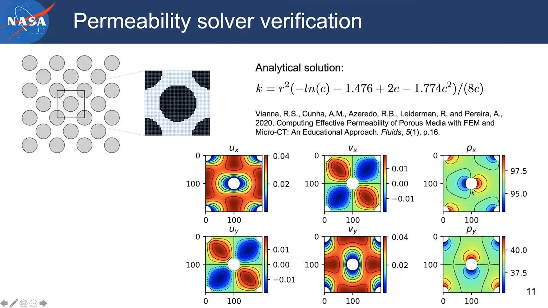
1. Permeability of an cylinder fiber array
import numpy as np
import pumapy as puma
import pyvista as pv
notebook = False # when running locally, actually open pyvista window
r = 0.1 # cylinder radius
vf = 2. * np.pi * (r ** 2.) # solid volume fraction
# The analytical solution can now be computed as:
keff_analytical = ((r ** 2) / (8 * vf)) * (-np.log(vf) - 1.47633597 + 2 * vf - 1.77428264 * vf ** 2 + 4.07770444 * vf ** 3 - 4.84227402 * vf ** 4)
print(f"Analytical diagonal permeability: {keff_analytical}")
# Create the square array of cylinders by running the following cell:
ws = puma.generate_cylinder_square_array(100, 1. - vf) # 100x100x1 domain with porosity = 1 - vf
ws.voxel_length = 1. / ws.matrix.shape[0] # i.e. side length = 1
print(f"Domain solid VF: {puma.compute_volume_fraction(ws, (1, 1))}")
puma.render_volume(ws, (1, 1), solid_color=(255, 255, 255), style='edges', notebook=notebook)
# Compute the numerical permeability tensor in 3D using a sparse direct solver
keff, (u_x, u_y, u_z) = puma.compute_permeability(ws, (1, 1), solver_type='direct')
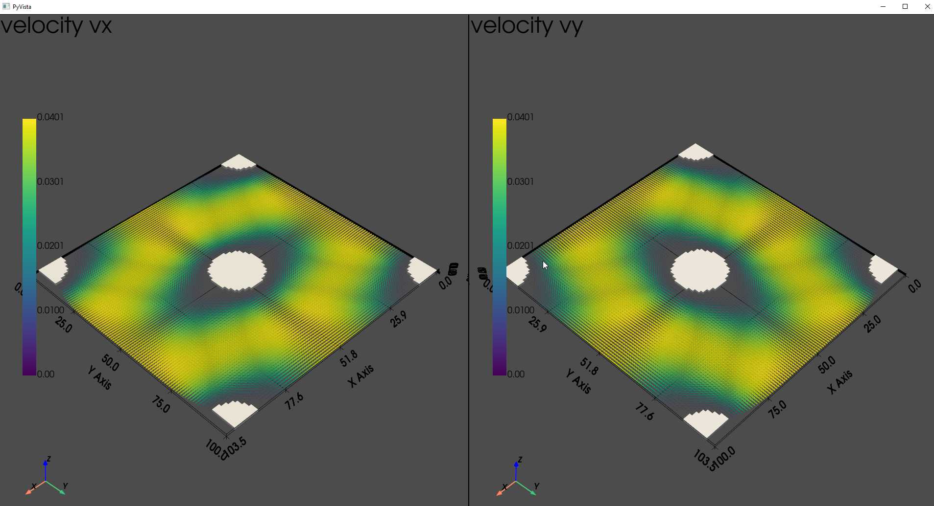
# We can also visualize the output velocity fields as:
p = pv.Plotter(shape=(1, 2))
ws.voxel_length = 1 # the voxel_length is converted to 1 for plotting the workspace together with the velocity
p.subplot(0, 0)
p.add_text("velocity vx")
puma.render_orientation(u_x, scale_factor=1e2, add_to_plot=p, plot_directly=False, notebook=notebook)
puma.render_volume(ws, (1, 1), solid_color=(255, 255, 255), style='surface', add_to_plot=p, plot_directly=False, notebook=notebook)
p.subplot(0, 1)
p.add_text("velocity vy")
puma.render_orientation(u_y, scale_factor=1e2, add_to_plot=p, plot_directly=False, notebook=notebook)
puma.render_volume(ws, (1, 1), solid_color=(255, 255, 255), style='surface', add_to_plot=p, plot_directly=False, notebook=notebook)
p.show()
The analytical solution:
$$
\begin{aligned}
U= & (F / 8 \pi \mu)\left[\ln (1 / \epsilon)-1.47633597+2 \epsilon-1.77428264 \epsilon^2\right. \\
& \left.+4.07770444 \epsilon^3-4.84227402 \epsilon^4+O\left(\epsilon^5\right)\right]
\end{aligned}
$$
From reference: Drummond J E, Tahir M I. Laminar viscous flow through regular arrays of parallel solid cylinders[J]. International Journal of Multiphase Flow, 1984, 10(5): 515-540.
2. Compute permeability of a textile REV
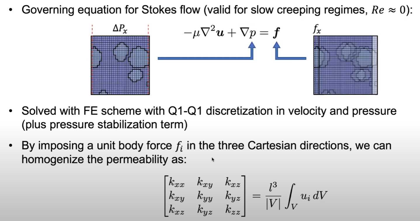
The numerical method behind the permeability homogenization function relies on a Finite Element method, which approximates both the velocity and pressure fields with first-order elements (i.e. Q1-Q1) and imposing a unit body force in each Cartesian direction. More details about the specifics of this method can be found in this publication, which was the starting point of the PuMA implementation.
Note:
- The file name of voxel model has to be followed by the number of voxels in x, y and z directions and splitted by "_".
- Only models discretized by square cubes (voxel) are supported in current version (V3.0).
import pumapy as puma
import pyvista as pv

notebook = False  # when running locally, actually open pyvista window

path = "./fabric_40_70_35.vtu"
ws = puma.import_weave_vtu(path, from_texgen_gui=True)
ws.voxel_length = 0.022e-3
puma.render_volume(ws, cutoff=(1, ws.matrix.max()), solid_color=None, notebook=notebook, cmap='jet', style='edges')

keff3, (u_x3, u_y3, u_z3) = puma.compute_permeability(ws, (1, ws.max()), tol=1e-8, maxiter=10000,
                                                      solver_type='minres', matrix_free=False)

p = pv.Plotter(shape=(2, 2), off_screen=False)

p.subplot(0, 0)
p.add_text("Fabric structure")
puma.render_volume(ws, cutoff=(1, ws.max()), cmap='jet', add_to_plot=p, plot_directly=False, notebook=notebook)

p.subplot(0, 1)
p.add_text("u_x")
puma.render_orientation(u_x3, add_to_plot=p, scale_factor=1e10, plot_directly=False)
puma.render_volume(ws, cutoff=(1, ws.max()), cmap='jet', add_to_plot=p, plot_directly=False, notebook=notebook)

p.subplot(1, 0)
p.add_text("u_y")
puma.render_orientation(u_y3, add_to_plot=p, scale_factor=1e10, plot_directly=False)
puma.render_volume(ws, cutoff=(1, ws.max()), cmap='jet', add_to_plot=p, plot_directly=False, notebook=notebook)

p.subplot(1, 1)
p.add_text("u_z")
puma.render_orientation(u_z3, add_to_plot=p, scale_factor=1e10, plot_directly=False)
puma.render_volume(ws, cutoff=(1, ws.max()), cmap='jet', add_to_plot=p, plot_directly=False, notebook=notebook)
p.show()
3. Another validation case
Session 12 Orientation Detection
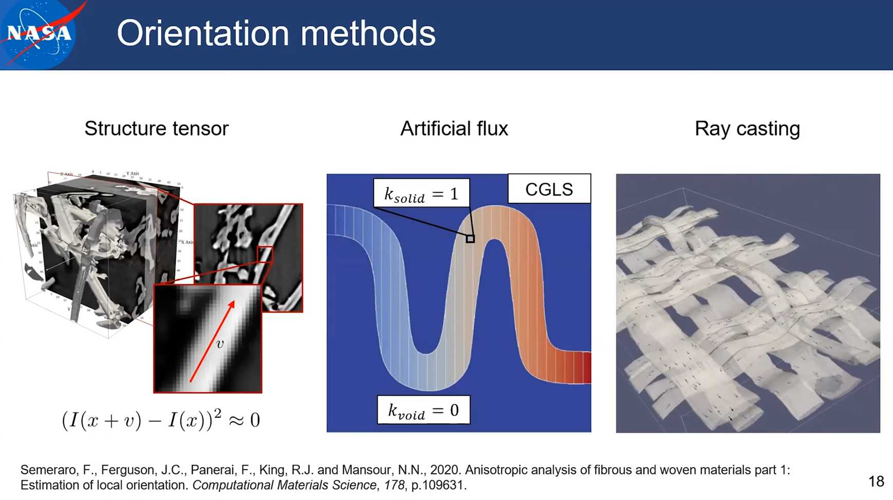
Note: the structure tensor method is available in pumapy and PuMA C++. The artificial flux and ray casting method are only available in C++ version of PuMA.
import pumapy as puma
import pyvista as pv
import os


notebook = False  # when running locally, actually open pyvista window

ws = puma.import_3Dtiff(puma.path_to_example_file("200_fiberform.tif"), 1.3e-6)

# sigma is the std of the DoG, whereas rho is the one of the second Gaussian smoothing
# in order to obtain optimal performance, we should always have:  sigma > rho
puma.compute_orientation_st(ws, cutoff=(90, 255), sigma=1.4, rho=0.7)

puma.export_vti("out/200_faberform.vti", ws)
Session 13 pumapy: Conductivity & Elasticity
Comments NOTHING