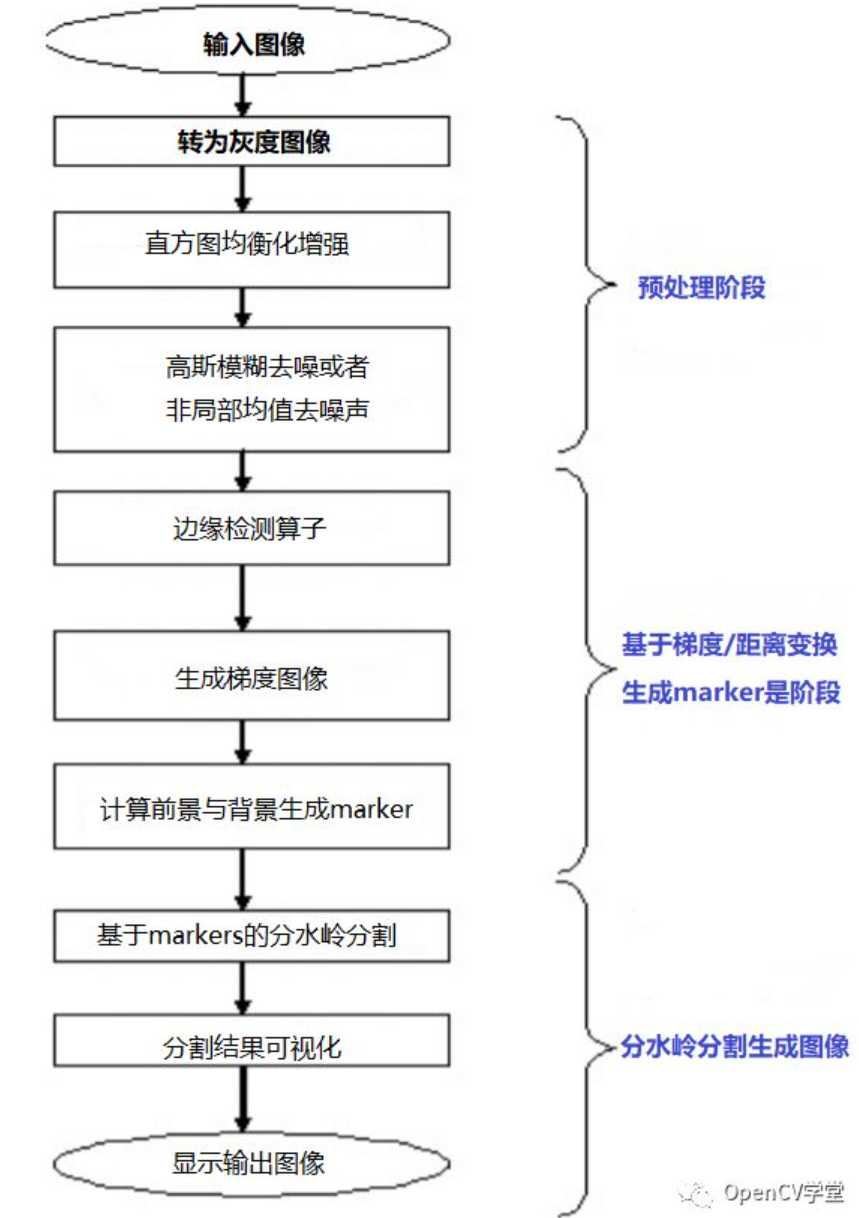
[PoreSpy]SNOW算法具体原理
在对图像进行消噪处理之后,CT灰度图的灰度值会趋于两极分化,取一定的阈值之后就可以将图像的明相和暗相即纤维区域和孔隙区域分割开来,在分离孔隙区域之后需要提取孔隙网络模型,孔隙网络模型包含若干个孔隙和喉道,SNOW算法就是对孔隙区域进行分割,然后分别提取孔隙和喉道,得到孔隙和喉道的位置几何参数
subnetwork of the oversegmented watershed (SNOW),是基于分水岭分割方法,提出的一种从高孔隙率材料中提取孔隙网络的算法。SNOW算法文献| Versatile and efficient pore network extraction method using marker-based watershed segmentation. Physical Review E, 96(2) | 10.1103/PhysRevE.96.023307
这是对分水岭算法的改进,分水岭算法的主要问题是,对于高孔隙率材料,距离变换不仅包含每个孔隙中心的峰值,还包含许多作为局部最大值出现的脊和平台(伪峰),这导致图像被过度分割。SNOW算法首先找到会导致过度分割分水岭的所有伪峰值,然后通过排除几个类别来逐步减少伪峰的数量,从而改善过度分割的问题
1.分水岭算法
这里讨论的是基于标记的分水岭算法,即通过对灰度图二值化之后,建立距离变换图像,找到距离变换峰值,根据峰值精准划分孔隙区域
相关理论可以参考:
OpenCV—图像分割中的分水岭算法原理与应用-CSDN博客
https://cloud.tencent.com/developer/article/1448221
为了更好地理解这个算法,考虑两个相互连接的孔隙的二值图像,如图1所示。假设对象的白色区域(孔隙区域)具有深度。每个像素的深度随着像素与最近的黑色像素的距离的增加而增加。这个深度就是距离变换,这个我们后面会说。
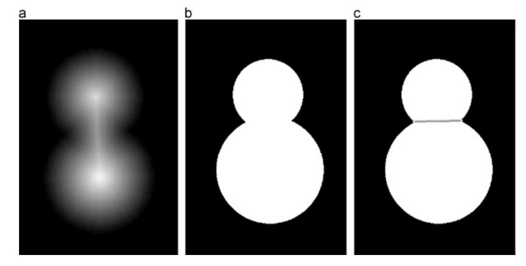
图1.两个孔隙的二值图像,分水岭方法的示例:(a)灰度值图,(b)原始二进制图像和(c)分割的孔隙。
将二值图像转换为距离变换图像后 -- 图2中,图像的距离变换很像地球表面的整个地理结构,每个像素的距离变换代表高度。其中的距离变换较大的像素连成的线可以看做山脊,也就是分水岭。其中的水就是二值化阈值,可以理解为水平面,比水平面低的区域会被淹没
刚开始用水填充每个孤立的山谷(局部最小值)。当水平面上升到一定高度时,水就会溢出当前山谷,可以通过在分水岭上修大坝,从而避免两个山谷的水汇集,这样图像就被分成2个像素集,一个是被水淹没的山谷像素集,一个是分水岭线像素集。最终这些大坝形成的线就对整个图像进行了分区,实现对图像的分割。通过水岭山脊线对孔隙区域进行分割,可以检测和提取两个相连的孔隙以及连接喉道。
分水岭算法的视频详解可以参考> chap7-watershed_哔哩哔哩_bilibili

图2.距离变换图。
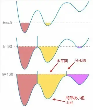
图3.分水岭算法演示过程。
2.距离变换
距离变换于1966年被学者首次提出,目前已被广泛应用于图像分析、计算机视觉、模式识别等领域,人们利用它来实现目标细化、骨架提取、形状插值及匹配、粘连物体的分离等。距离变换是针对二值图像的一种变换。在二维空间中,一幅二值图像可以认为仅仅包含目标和背景两种像素(在这里可以认为孔隙区域为目标,固体骨架位区域背景),目标的像素值为1,背景的像素值为0;距离变换的结果不是另一幅二值图像,而是一幅灰度级图像,即距离图像,图像中目标区域的每个像素的距离值为该像素与距其最近的背景像素间的距离。
距离变换按照距离的类型可以分为欧式距离变换(Eudlidean Distance Transfrom)和非欧式距离变换两种,其中,非欧式距离变换又包括棋盘距离变换(Chessboard Distance Transform),城市街区距离变换(Cityblock Distance Transform)等
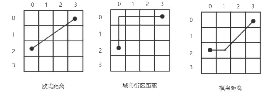
图4.几种常见距离变换的原理图。
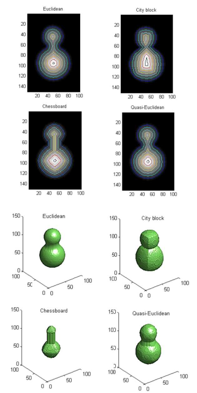
图5.不同距离变换下图像分割后的形状。
上面两个图演示了不同距离变化算法下经分水岭分割后的2D,3D图,可以看到四种距离变换均能较好的体现孔隙的形状,但是只有棋盘距离变换较好的体现出了喉道的形状,出处如下:
在对多孔介质二值化图像进行距离变换处理后,参考下图,图像大小为400 × 400,白色圆盘半径为10像素,其余部分为孔隙。虽然简单,但这种几何形状足以说明本基本分水岭方法存在的问题
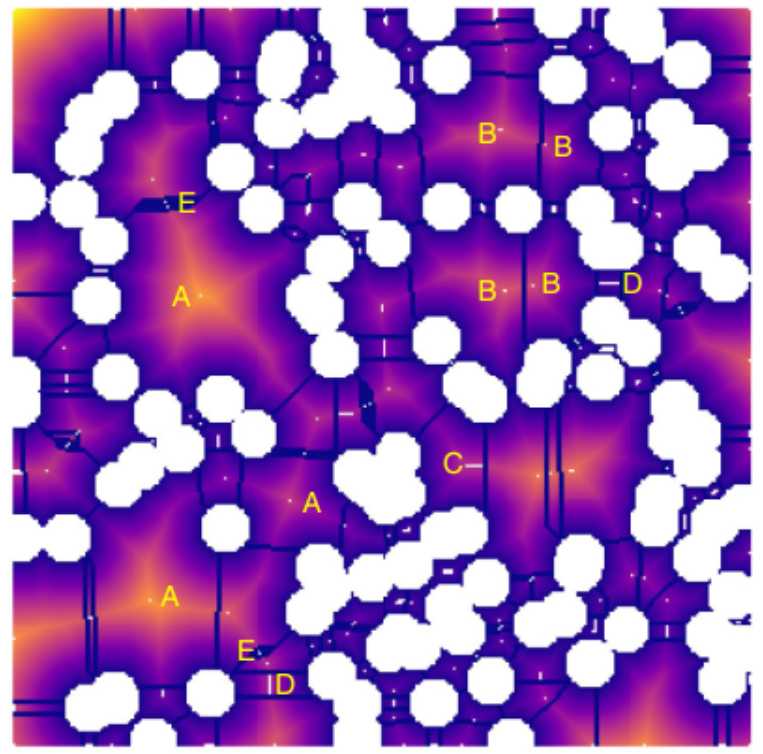
图6.分水岭分割后的距离变化图,高亮区域为孔隙区域,高亮点为距离变化峰值。
图中的几个高亮区域表示孔隙,亮度越高表面该位置的像素距离固体骨架越远,高亮点为距离变换的峰值,可以观察到有些地方的峰值位置过近,比如B区域,两个峰值完全可以合并成一个,C和D区域的峰值甚至直接连成一条线段,E区域也出现细小峰值团簇的现象。
出现这种问题的原因在于基本分水岭算法的通病,那就是过度分割,距离变换图像看作地形图也会有许多小的杂峰或是峰之间的鞍点,这些杂峰在分水岭分割时也会被单独划分出来,就出现了上图中许多峰聚集在一起的问题,解决办法就是消除杂峰和鞍点,这也是SNOW算法较分水岭算法的优势
3.SNOW算法
这里主要讲SNOW算法如何去除杂峰和鞍点
3.1 去除杂峰
距离变化图像和灰度图类似,都是给每个像素点分配一个固定的值,同样距离变化图也会有噪声,即杂峰。和处理灰度图的噪声一样,消除距离变化杂峰的办法就是应用各种过滤器,在SNOW算法文献中用的是高斯滤波器
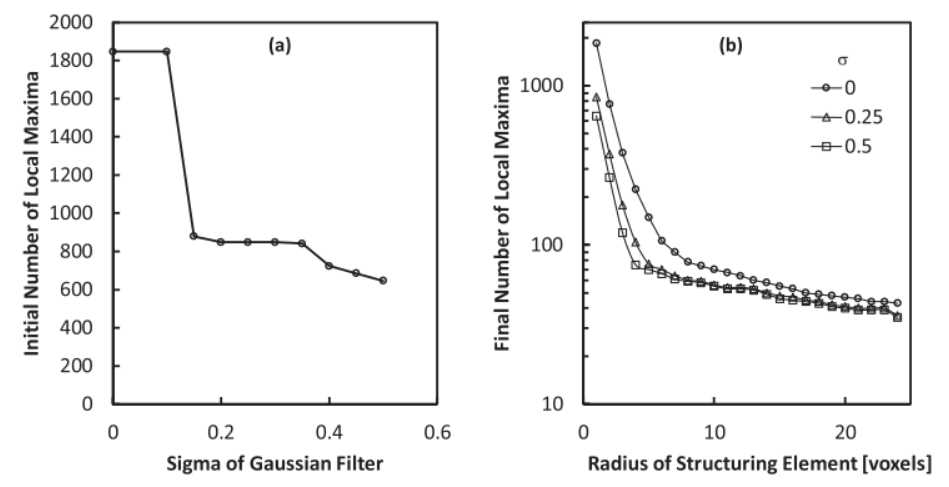
图7.高斯滤波器不同标准差和模糊半径对峰值数量的影响。
3.2 去除鞍点峰值
去除杂峰之后,下一步就是消除位于距离图的鞍和平原上的假峰。这些峰被错误地识别出来,因为它们被几个具有相同距离值的体素包围,但随着脊向开放孔隙空间延伸,它们最终连接到具有更高值的体素;如图8(a)和8(b)所示。
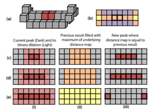
图8.去除鞍点峰的原理示意图。
如图8(c) -8 (e)所示。每个峰分别使用以下迭代过程进行分析:在步骤(i)中,用最小立方结构元素(3N−dim)体素扩展峰。然后,这个扩大的峰值被步骤(ii)中所示的底层距离图中的最大值淹没。
最后,将淹水膨胀图与距离图进行比较,并将这两幅图中所有相等的体素视为新峰(s) (iii)。在重复上述步骤之前,将新峰与旧峰进行比较。如果旧峰是新峰的子集,如图8(c-iii)和8(d-iii)所示,则重复步骤(i) - (iii)。如果它们是相同的,那么这个峰值是一个真正的局部最大值,搜索停止。
如果旧峰不是新峰的子集,如图8(e-iii)所示,则旧峰为鞍点,结束搜索。然后从原始峰图像中去除这些峰
代码展示如下
import scipy as sp
import numpy as np
import scipy.ndimage as spim
import scipy.spatial as sptl
import matplotlib.pyplot as plt
from skimage.morphology import watershed
from skimage.feature import peak_local_max
from skimage.segmentation import find_boundaries
#与膨胀算法类似,把目标位置的边框扩大
def extend_slice(slices, shape, pad=1):
    """
    调整切片索引以扩大切片区域.

    同时进行边界检索,确保切片区域不会扩张到图片外.

    Parameters
    ----------
    slices : 切片对象列表
         N个切片组成的列表或者元组, N是图像的维度.
    shape : array_like
        切片对象应用到的图像的形状。这用于检查边界,以防止索引超出图像.
    pad : int or list of ints
        在每个方向上要扩展的体素数。

    Returns
    -------
    slices : list of slice objects
        切片对象的列表,其start和stop值分别递增和递减1,不超出图像边界。

    Examples
    --------
    >>> from scipy.ndimage import label, find_objects
    >>> from porespy.tools import extend_slice
    >>> im = np.array([[1, 0, 0], [1, 0, 0], [0, 0, 1]])
    >>> labels = label(im)[0]
    >>> s = find_objects(labels)

    使用 find_objects函数返回的切片,将第一个标签设置为3

    >>> labels[s[0]] = 3
    >>> print(labels)
    [[3 0 0]
     [3 0 0]
     [0 0 2]]

    扩展切片,并将切片区域内的value改为4

    >>> s_ext = extend_slice(s[0], shape=im.shape, pad=1)
    >>> labels[s_ext] = 4
    >>> print(labels)
    [[4 4 0]
     [4 4 0]
     [4 4 2]]

    从4的位置可以看出,切片被扩展了1,并且正确地处理了超出边界的扩展

    Examples
    --------
    `Click here
    `_
    to view online example.

    """
    shape = np.array(shape)
    pad = np.array(pad).astype(int)*(shape > 0)
    a = []
    for i, s in enumerate(slices):
        start = 0
        stop = shape[i]
        start = max(s.start - pad[i], 0)
        stop = min(s.stop + pad[i], shape[i])
        a.append(slice(start, stop, None))
    return tuple(a)

#运行迭代运算,每次迭代过程中对峰值像素的位置区域进行扩张,将扩张后区域内所有像素的距离变换值赋予为峰值,对比扩张前后的距离变换图
#扩张前为扩张后的子集则继续迭代,扩张前后相等则原峰值为真正的局部峰值,扩张前后不等则原峰值为鞍点,删除鞍点,迭代停止
def trim_saddle_points_legacy(peaks, dt, maxiter=10):
    """
    去除在距离变换中被错误识别的鞍点或山脊上的峰

    Parameters
    ----------
    peaks : ND-array
        包含True值的布尔图像,用于标记距离变换中的峰值的位置 (``dt``)
    dt : ND-array
        图像孔隙区域的距离变换图(固体骨架区域为背景).
    maxiter : int
        识别并删除鞍点时要运行的最大迭代数。默认值是10,通常不会达到这个值;但是,如果在移除所有鞍点之前循环结束,则会发出警告。

    Returns
    -------
    image : ND-array
        An image with fewer peaks than the input image

    Notes
    -----
    This version of the function was included in versions of PoreSpy = 2.
    This is included here for legacy reasons

    References
    ----------
    [1] Gostick, J. "A versatile and efficient network extraction algorithm
    using marker-based watershed segmenation".  Physical Review E. (2017)

    Examples
    --------
    `Click here
    `_
    to view online example.
    """
    new_peaks = np.zeros_like(peaks, dtype=bool)
    if dt.ndim == 2:
        from skimage.morphology import square as cube
    else:
        from skimage.morphology import cube
    labels, N = spim.label(peaks > 0)#求解距离变换峰值的邻域,默认为峰值相连的上下左右四个像素
    slices = spim.find_objects(labels)#标记邻域的边界框,找到峰所在区域
    for i, s in tqdm(enumerate(slices), **settings.tqdm):
        sx = extend_slice(s, shape=peaks.shape, pad=10)#峰值区域扩张
        peaks_i = labels[sx] == i + 1
        dt_i = dt[sx]
        im_i = dt_i > 0
        iters = 0
        while iters = maxiter:
            logger.debug(
                "Maximum number of iterations reached, consider "
                + "running again with a larger value of max_iters"
            )
    return new_peaks*peaks
3.3 去除相距较近的峰值
从图6 B区域可以看到明明可以合并成一个峰的区域出现了两个峰值,这也是过度分割的一个原因,处理方法很简单
在算法上,通过找到(a)每对峰之间的距离 ,(b)每个峰的距离变换值,比较a,b的大小来识别这些峰。当发现a<b时,则保留距离斌换最大的那个峰。
如果图像有N个峰,则距离矩阵为N × N矩阵,其中峰i与峰j之间的距离存储在元素(i, j)中。因此,对于峰i,可以通过在第i行搜索低于峰i的距离图值的距离值来识别满足条件的峰。代码如下
def trim_nearby_peaks(peaks, dt, f=1):
    """
    移除相距较近的峰对中,离背景较近的峰

    Parameters
    ----------
    peaks : ndarray
        包含非零值的图像,表示距离变换( dt )中的峰值。如果 peaks 是布尔值,则返回一个布尔值;如果peaks 已经被标记,则返回原始标签,不包含修剪过的峰.
    dt : ndarray
        孔隙区域的距离变换图像
    f : scalar
        判断两个峰间距足够小可以被认定为峰对的距离,如果``d_neighbor < f * d_solid``则认为峰距过近.

    Returns
    -------
    image : ndarray
       与“peaks”大小和类型相同的矩阵,包含原始图像中峰值的子集。


    Notes
    -----
    如果有三个峰相距较近,考虑每对。这样可以确保只保留离固体最远的单个峰值。不需要迭代。


    References
    ----------
    [1] Gostick, J. "A versatile and efficient network extraction
    algorithm using marker-based watershed segmenation". Physical Review
    E. (2017)

    Examples
    --------
    `Click here
    `_
    to view online example.

    """
    if dt.ndim == 2:
        from skimage.morphology import square as cube
    else:
        from skimage.morphology import cube

    labels, N = spim.label(peaks > 0, structure=cube(3))
    crds = spim.measurements.center_of_mass(peaks > 0, labels=labels,
                                            index=np.arange(1, N + 1))
    crds = np.vstack(crds).astype(int)  # Convert to numpy array of ints
    L = dt[tuple(crds.T)]  # Get distance to solid for each peak
    # Add tiny amount to joggle points to avoid equal distances to solid
    # arange was added instead of random values so the results are repeatable
    L = L + np.arange(len(L))*1e-6

    tree = sptl.KDTree(data=crds)
    # Find list of nearest peak to each peak
    temp = tree.query(x=crds, k=2)
    nearest_neighbor = temp[1][:, 1]
    dist_to_neighbor = temp[0][:, 1]
    del temp, tree  # Free-up memory
    hits = np.where(dist_to_neighbor <= f * L)[0]
    # Drop peak that is closer to the solid than it's neighbor
    drop_peaks = []
    for i in hits:
        if L[i] < L[nearest_neighbor[i]]:
            drop_peaks.append(i)
        else:
            drop_peaks.append(nearest_neighbor[i])
    drop_peaks = np.unique(drop_peaks)

    new_peaks = ~np.isin(labels, drop_peaks+1)*peaks
    return new_peaks
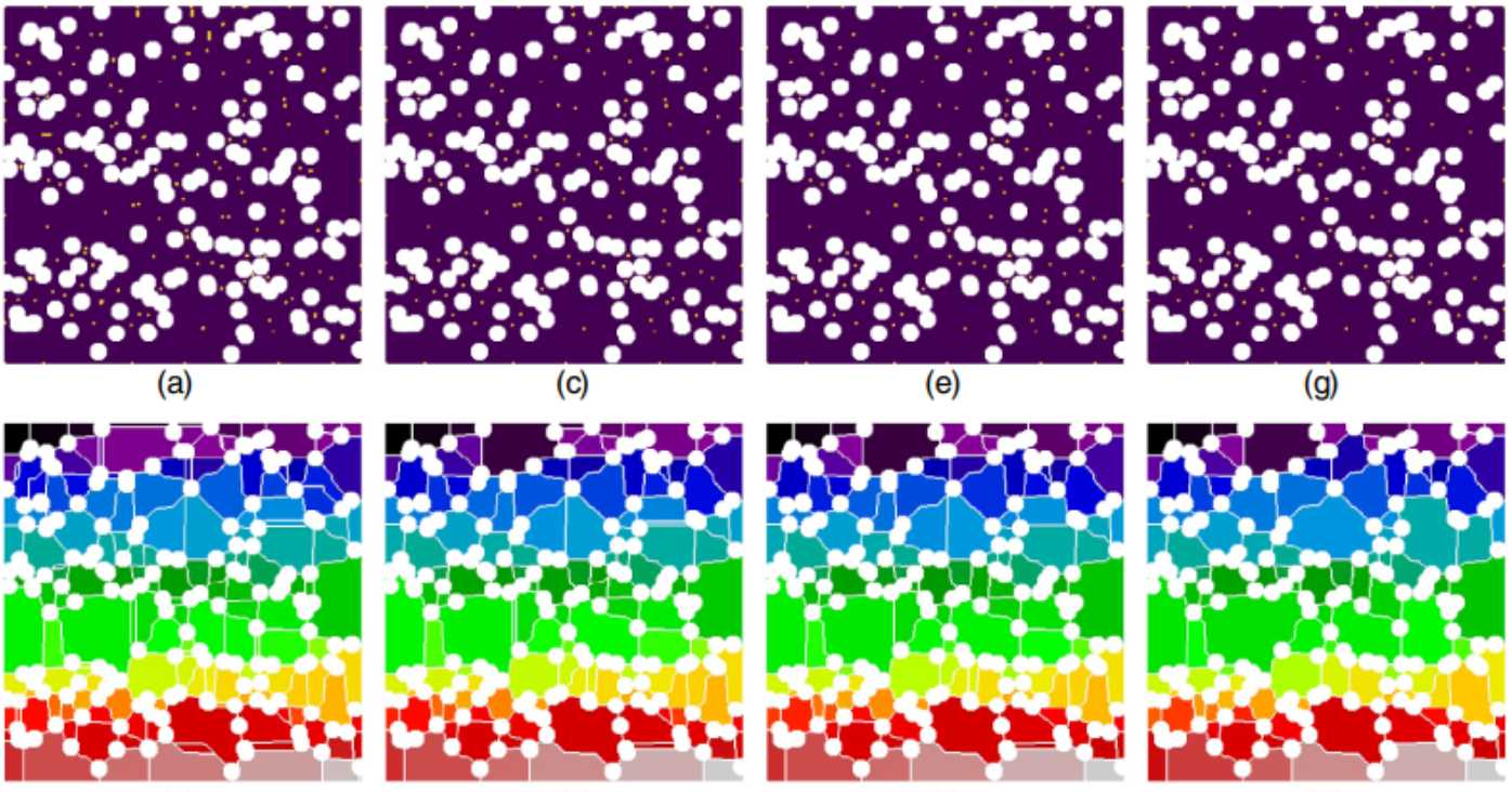
图9.SNOW算法处理杂峰的效果演示。
上图是用于去除杂散峰值的SNOW算法的图示。顶行显示了每一步的距离变换峰值,底行显示了孔隙空间的分割结果。伪峰值的逐渐消除可以从左到右看到。距离变换的高斯模糊产生了最显著的改进[列2(c),(d)]。鞍点的消除去除了孔隙之间的薄区域[第3列(e)、(f)]。彼此靠近的合并峰防止了大的连续区域的平分[第4列(g)、(h)]。
4 孔隙网络模型几何参数的提取
SNOW算法的最后一步是从分割好的孔隙区域中提取孔隙和喉道的信息,主要方法是基于距离变换图中的体素集来获得孔隙网络模型的几何信息
要确定孔隙i的大小、体积、位置等,只需对标记为i的体素的分水岭图像区域进行隔离,并分析该区域的属性,如图10(b) - (d)所示。
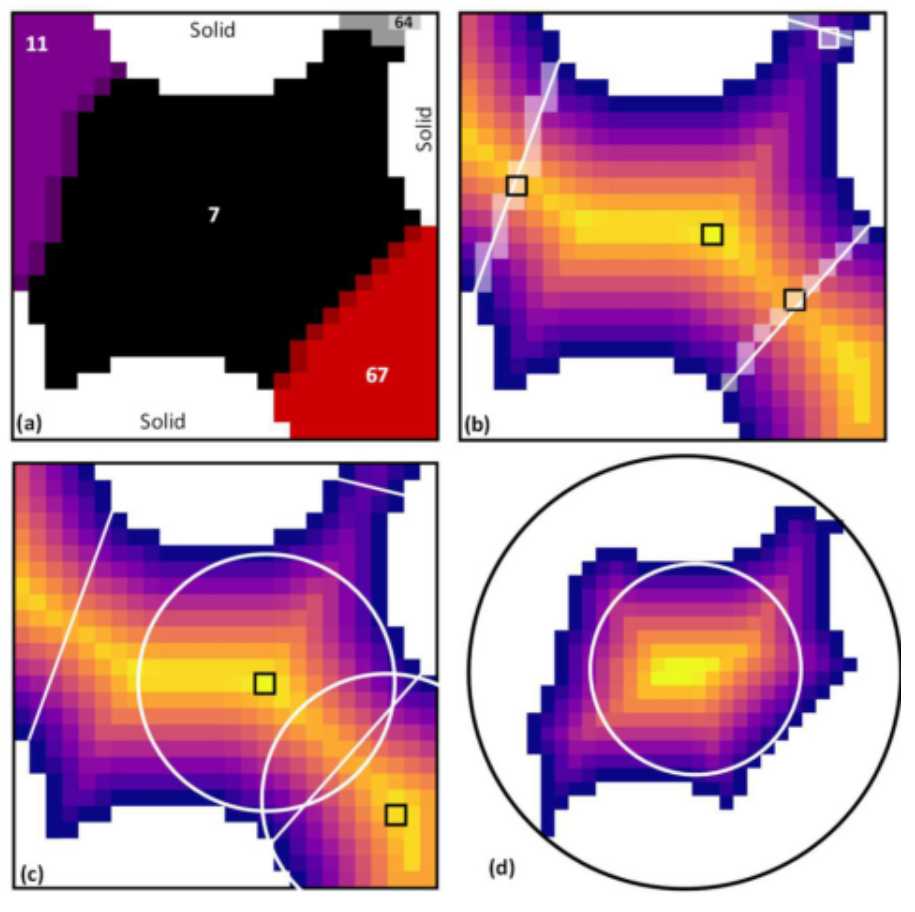
图10.二维孔隙的连通性和大小测定图。
上图中(a)包含4个孔隙区域标记分别是7,11,64,67。喉道区域是通过扩大各个孔隙区域并识别重叠区域来发现的,用浅色像素表示。(b)对图像进行距离变换,从黑框表示的峰值确定喉道大小信息。(c)使用全局距离图的结果是孔隙直径延伸到邻近的孔隙。
(d)使用在孔隙内获得的距离图只能得到内切孔径和几何上更一致的孔隙质心。
下面说一下算法提取的孔隙网络模型的几何参数有哪些:
Pore-Volume:孔隙区域的体积可以通过将该区域内的体素数相加得到[即图10(a)中所有的黑色体素]。该值不是通过孔隙半径计算的球的体积值
Pore-Extended diameter:该值作为每个孔隙区域内的全局距离图的最大值。如图10(c)所示,该定义意味着孔径可以延伸到邻近的孔隙中。这些扩展的孔隙往往相互重叠,从而产生问题,例如负的喉道长度和孔隙体积的重复计算
Pore-Inscribed diameter:这是通过与扩展直径相同的方式获得的,但只使用孔隙区域的局部距离图。如图6(d)所示,这将孔隙体完全限制在其区域内。除非另有说明,否则在所有计算中都使用该值作为孔径。
Pore-Surface area:在体素图像中,面积的计算是相当困难的。计算一个体积表面上的体素数很简单,但要知道它代表多少面积就不那么简单了。表面体素的数量是在局部距离变换中具有值为1的体素的数量。在Dong和Blunt之后,面积估计为表面上的体素数乘以一个体素面面积。
H. Dong and M. J. Blunt, Pore-network extraction from microcomputerized-tomography images, Phys. Rev. E 80, 036307 (2009).
Pore-Coordinates:孔隙坐标是峰值在全局或局部距离图中的位置,也可以作为区域的质心。这里使用的是后者,因为在距离图中找到峰值是一个复杂的问题,如上所述。这种选择意味着孔径值不一定与孔中心位置对应,但位移较小。
Throat-Inscribed diameter:如图10(b)所示,可以从全局距离变换的最大值中识别出喉部直径。
Throat-Total length:两个孔之间的总长度计算为两个孔的质心通过喉部质心之间的欧氏距离
Throat-Direct length:两个孔中心之间不通过喉形心的直线上的长度
Throat-Connect:对每个孔隙区域进行膨胀算法(切片扩张)当两个孔隙扩张之后存在交集,那么就判断这两个孔隙是相连的
提取孔隙网络模型几何信息的代码如下:
def regions_to_network(regions, phases=None, voxel_size=1, accuracy='standard'):
    r"""
    Analyzes an image that has been partitioned into pore regions and extracts
    the pore and throat geometry as well as network connectivity.

    Parameters
    ----------
    regions : ndarray
        An image of the material partitioned into individual regions.
        Zeros in this image are ignored.
    phases : ndarray, optional
        An image indicating to which phase each voxel belongs. The returned
        network contains a 'pore.phase' array with the corresponding value.
        If not given a value of 1 is assigned to every pore.
    voxel_size : scalar (default = 1)
        The resolution of the image, expressed as the length of one side of a
        voxel, so the volume of a voxel would be **voxel_size**-cubed.
    accuracy : string
        Controls how accurately certain properties are calculated. Options are:

        'standard' (default)
            Computes the surface areas and perimeters by simply counting
            voxels.  This is *much* faster but does not properly account
            for the rough, voxelated nature of the surfaces.
        'high'
            Computes surface areas using the marching cube method, and
            perimeters using the fast marching method.  These are substantially
            slower but better account for the voxelated nature of the images.

    Returns
    -------
    net : dict
        A dictionary containing all the pore and throat size data, as well as
        the network topological information.  The dictionary names use the
        OpenPNM convention (i.e. 'pore.coords', 'throat.conns').

    Notes
    -----
    The meaning of each of the values returned in ``net`` are outlined below:

    'pore.region_label'
        The region labels corresponding to the watershed extraction. The
        pore indices and regions labels will be offset by 1, so pore 0
        will be region 1.
    'throat.conns'
        An *Nt-by-2* array indicating which pores are connected to each other
    'pore.region_label'
        Mapping of regions in the watershed segmentation to pores in the
        network
    'pore.local_peak'
        The coordinates of the location of the maxima of the distance transform
        performed on the pore region in isolation
    'pore.global_peak'
        The coordinates of the location of the maxima of the distance transform
        performed on the full image
    'pore.geometric_centroid'
        The center of mass of the pore region as calculated by
        ``skimage.measure.center_of_mass``
    'throat.global_peak'
        The coordinates of the location of the maxima of the distance transform
        performed on the full image
    'pore.region_volume'
        The volume of the pore region computed by summing the voxels
    'pore.volume'
        The volume of the pore found by as volume of a mesh obtained from the
        marching cubes algorithm
    'pore.surface_area'
        The surface area of the pore region as calculated by either counting
        voxels or using the fast marching method to generate a tetramesh (if
        ``accuracy`` is set to ``'high'``.)
    'throat.cross_sectional_area'
        The cross-sectional area of the throat found by either counting
        voxels or using the fast marching method to generate a tetramesh (if
        ``accuracy`` is set to ``'high'``.)
    'throat.perimeter'
        The perimeter of the throat found by counting voxels on the edge of
        the region defined by the intersection of two regions.
    'pore.inscribed_diameter'
        The diameter of the largest sphere inscribed in the pore region. This
        is found as the maximum of the distance transform on the region in
        isolation.
    'pore.extended_diameter'
        The diamter of the largest sphere inscribed in overal image, which
        can extend outside the pore region. This is found as the local maximum
        of the distance transform on the full image.
    'throat.inscribed_diameter'
        The diameter of the largest sphere inscribed in the throat.  This
        is found as the local maximum of the distance transform in the area
        where to regions meet.
    'throat.total_length'
        The length between pore centered via the throat center
    'throat.direct_length'
        The length between two pore centers on a straight line between them
        that does not pass through the throat centroid.

    Examples
    --------
    `Click here
    `_
    to view online example.

    """
    logger.info('Extracting pore/throat information')

    im = make_contiguous(regions)
    struc_elem = disk if im.ndim == 2 else ball
    voxel_size = float(voxel_size)
    if phases is None:
        phases = (im > 0).astype(int)
    if im.size != phases.size:
        raise Exception('regions and phase are different sizes, probably ' +
                        'because boundary regions were not added to phases')
    dt = np.zeros_like(phases, dtype="float32")  # since edt returns float32
    for i in np.unique(phases[phases.nonzero()]):
        dt += edt(phases == i)

    # Get 'slices' into im for each pore region
    slices = spim.find_objects(im)

    # Initialize arrays
    Ps = np.arange(1, np.amax(im)+1)
    Np = np.size(Ps)
    p_coords_cm = np.zeros((Np, im.ndim), dtype=float)
    p_coords_dt = np.zeros((Np, im.ndim), dtype=float)
    p_coords_dt_global = np.zeros((Np, im.ndim), dtype=float)
    p_volume = np.zeros((Np, ), dtype=float)
    p_dia_local = np.zeros((Np, ), dtype=float)
    p_dia_global = np.zeros((Np, ), dtype=float)
    p_label = np.zeros((Np, ), dtype=int)
    p_area_surf = np.zeros((Np, ), dtype=int)
    p_phase = np.zeros((Np, ), dtype=int)
    # The number of throats is not known at the start, so lists are used which can be dynamically resized more easily.
    t_conns = []
    t_dia_inscribed = []
    t_area = []
    t_perimeter = []
    t_coords = []

    # Start extracting size information for pores and throats
    msg = "Extracting pore and throat properties"
    for i in tqdm(Ps, desc=msg, **settings.tqdm):
        pore = i - 1
        if slices[pore] is None:
            continue
        s = extend_slice(slices[pore], im.shape)
        sub_im = im[s]
        sub_dt = dt[s]
        pore_im = sub_im == i
        padded_mask = np.pad(pore_im, pad_width=1, mode='constant')
        pore_dt = edt(padded_mask)
        s_offset = np.array([i.start for i in s])
        p_label[pore] = i
        p_coords_cm[pore, :] = spim.center_of_mass(pore_im) + s_offset
        temp = np.vstack(np.where(pore_dt == pore_dt.max()))[:, 0]
        p_coords_dt[pore, :] = temp + s_offset
        p_phase[pore] = (phases[s]*pore_im).max()
        temp = np.vstack(np.where(sub_dt == sub_dt.max()))[:, 0]
        p_coords_dt_global[pore, :] = temp + s_offset
        p_volume[pore] = np.sum(pore_im, dtype=np.int64)
        p_dia_local[pore] = 2*np.amax(pore_dt)
        p_dia_global[pore] = 2*np.amax(sub_dt)
        # The following is overwritten if accuracy is set to 'high'
        p_area_surf[pore] = np.sum(pore_dt == 1, dtype=np.int64)
        im_w_throats = spim.binary_dilation(input=pore_im, structure=struc_elem(1))
        im_w_throats = im_w_throats*sub_im
        Pn = np.unique(im_w_throats)[1:] - 1
        for j in Pn:
            if j > pore:
                t_conns.append([pore, j])
                vx = np.where(im_w_throats == (j + 1))
                t_dia_inscribed.append(2*np.amax(sub_dt[vx]))
                # The following is overwritten if accuracy is set to 'high'
                t_perimeter.append(np.sum(sub_dt[vx] < 2, dtype=np.int64))
                # The following is overwritten if accuracy is set to 'high'
                t_area.append(np.size(vx[0]))
                p_area_surf[pore] -= np.size(vx[0])
                t_inds = tuple([i+j for i, j in zip(vx, s_offset)])
                temp = np.where(dt[t_inds] == np.amax(dt[t_inds]))[0][0]
                t_coords.append(tuple([t_inds[k][temp] for k in range(im.ndim)]))

    # Clean up values
    p_coords = p_coords_cm
    Nt = len(t_dia_inscribed)  # Get number of throats
    if im.ndim == 2:  # If 2D, add 0's in 3rd dimension
        p_coords = np.vstack((p_coords_cm.T, np.zeros((Np, )))).T
        t_coords = np.vstack((np.array(t_coords).T, np.zeros((Nt, )))).T

    net = {}
    ND = im.ndim
    # Define all the fundamental stuff
    net['throat.conns'] = np.array(t_conns)
    net['pore.coords'] = np.array(p_coords)*voxel_size
    net['pore.all'] = np.ones_like(net['pore.coords'][:, 0], dtype=bool)
    net['throat.all'] = np.ones_like(net['throat.conns'][:, 0], dtype=bool)
    net['pore.region_label'] = np.array(p_label)
    net['pore.phase'] = np.array(p_phase, dtype=int)
    net['throat.phases'] = net['pore.phase'][net['throat.conns']]
    V = np.copy(p_volume)*(voxel_size**ND)
    net['pore.region_volume'] = V  # This will be an area if image is 2D
    f = 3/4 if ND == 3 else 1.0
    net['pore.equivalent_diameter'] = 2*(V/np.pi * f)**(1/ND)
    # Extract the geometric stuff
    net['pore.local_peak'] = np.copy(p_coords_dt)*voxel_size
    net['pore.global_peak'] = np.copy(p_coords_dt_global)*voxel_size
    net['pore.geometric_centroid'] = np.copy(p_coords_cm)*voxel_size
    net['throat.global_peak'] = np.array(t_coords)*voxel_size
    net['pore.inscribed_diameter'] = np.copy(p_dia_local)*voxel_size
    net['pore.extended_diameter'] = np.copy(p_dia_global)*voxel_size
    net['throat.inscribed_diameter'] = np.array(t_dia_inscribed)*voxel_size
    P12 = net['throat.conns']
    PT1 = np.sqrt(np.sum(((p_coords[P12[:, 0]]-t_coords)*voxel_size)**2,
                         axis=1))
    PT2 = np.sqrt(np.sum(((p_coords[P12[:, 1]]-t_coords)*voxel_size)**2,
                         axis=1))
    net['throat.total_length'] = PT1 + PT2
    PT1 = PT1-p_dia_local[P12[:, 0]]/2*voxel_size
    PT2 = PT2-p_dia_local[P12[:, 1]]/2*voxel_size
    dist = (p_coords[P12[:, 0]] - p_coords[P12[:, 1]])*voxel_size
    net['throat.direct_length'] = np.sqrt(np.sum(dist**2, axis=1, dtype=np.int64))
    net['throat.perimeter'] = np.array(t_perimeter)*voxel_size
    if (accuracy == 'high') and (im.ndim == 2):
        msg = "accuracy='high' only available in 3D, reverting to 'standard'"
        logger.warning(msg)
        accuracy = 'standard'
    if (accuracy == 'high'):
        net['pore.volume'] = region_volumes(regions=im, mode='marching_cubes')
        areas = region_surface_areas(regions=im, voxel_size=voxel_size)
        net['pore.surface_area'] = areas
        interface_area = region_interface_areas(regions=im, areas=areas,
                                                voxel_size=voxel_size)
        A = interface_area.area
        net['throat.cross_sectional_area'] = A
        net['throat.equivalent_diameter'] = (4*A/np.pi)**(1/2)
    else:
        net['pore.volume'] = np.copy(p_volume)*(voxel_size**ND)
        net['pore.surface_area'] = np.copy(p_area_surf)*(voxel_size**2)
        A = np.array(t_area)*(voxel_size**2)
        net['throat.cross_sectional_area'] = A
        net['throat.equivalent_diameter'] = (4*A/np.pi)**(1/2)

    return net
Comments NOTHING