Please refresh the page if equations are not rendered correctly.
---------------------------------------------------------------

一 理论基础

本文提供与流体力学和计算流体力学（CFD）有关的张量数学信息。 它描述了标量和向量以及典型的代数向量操作。 接下来是二阶张量、它们的代数运算、对称性、偏度和张量不变量，如迹和行列式。 在描述坐标系和轴的转换之前，它简要地讨论了高揭张量。 介绍了张量计算，以及导数运算符，如div、grad、curl和Laplacian。 最后一节包括高斯和斯托克斯的积分定理，以及div和curl的物理表示，还有标量和向量势（scalar and vector potentials）。

1. 标量与向量¹

标量是任何可以用某个选定的单位系统中的单一实数表示的物理属性，例如压力（kg/(m \cdot s^2)）、温度（K）和密度（kg/m^3 ）。标量用斜体单字母表示，如p、T、ρ。标量运算必须使用一致的单位；特别是加法、减法和相等只对相同维度单位的标量有物理意义。

向量是一个包含大小和方向信息的实体。在其最一般的形式中，一个n维向量\mathbf{a}可以由n个标量分量(a_1,a_2,...a_n)表示，对应于坐标轴x_1 , x_2，...，x_n。在连续介质力学中，我们处理的问题一般都处于三维（欧几里得）空间，因此，向量\mathbf{a} = (a_1, a_2, a_3)与一组坐标轴x_1, x_2, x_3相对应。在矩形笛卡尔坐标系中，这组坐标轴是x, y, z（见4.1节），在圆柱和球面极坐标系中则分别代表r, θ, z和r, θ, j。因此，即使坐标系不同，一个向量总是可以使用索引为i的向量标记a_i(i = 1, 2, ..., n)表示，其中i对应于每个坐标轴。索引i在数学文本中通常被省略，因为它暗含在方程的书写形式之中。在本文中，向量或张量（见第2节）用黑体字母表示，如\mathbf{a}。这种符号的好处是：它不暗示任何关于坐标系的东西。因此，它增强了向量作为一个有方向和大小的实体的概念，而不是一组三个标量；而且，它更紧凑。

一个向量a或a_i的大小或模在各自的符号中用|a|和a表示。单位大小的向量被称为单位向量。本文假设读者熟悉向量和标量的乘法以及向量的加减法等基本运算。这些运算都是满足结合律和交换律的。接下来的三节描述了连续介质力学中需要的其余向量和张量操作。

1.1 符号约定

处理方程的一种常见且简单的方法是使用向量表示法而不是爱因斯坦求和约定。 向量符号需要有关特殊数学的知识。 因此，现在给出应用于标量、向量和张量的不同操作的简要描述。 为此，现在定义任意量：一个标量\phi，两个向量 \mathbf{a} 和\mathbf{b} 以及一个张量\mathbf{T}：

\mathbf{a}=\left(\begin{array}{l}
a_{x} \\
a_{y} \\
a_{z}
\end{array}\right)=\left(\begin{array}{l}
a_{1} \\
a_{2} \\
a_{3}
\end{array}\right)

\mathbf{b}=\left(\begin{array}{l}
b_{x} \\
b_{y} \\
b_{z}
\end{array}\right)=\left(\begin{array}{l}
b_{1} \\
b_{2} \\
b_{3}
\end{array}\right)

\mathbf{T}=\left[\begin{array}{lll}
T_{x x}&T_{x y}&T_{x z} \\
T_{y x}&T_{y y}&T_{y z} \\
T_{z x}&T_{z y}&T_{z z}
\end{array}\right]=\left[\begin{array}{lll}
T_{11}&T_{12}&T_{13} \\
T_{21}&T_{22}&T_{23} \\
T_{31}&T_{32}&T_{33}
\end{array}\right] .

根据感兴趣的操作，我们可以选用数字（1，2，3）或空间坐标分量（x，y，z）作为二阶张量元素的下标。单位向量\mathbf{e}_i和的定义如下：

\mathbf{e}_1 = \mathbf{e}_x = \left( \begin{array}{l}
1 \\
0 \\
0
\end{array}\right)

\mathbf{e}_2=\mathbf{e}_y=\left(\begin{array}{l}
0 \\
1 \\
0
\end{array}\right)

\mathbf{e}_3=\mathbf{e}_z=\left(\begin{array}{l}
0 \\
0 \\
1
\end{array}\right)

此外，单位向量单位矩阵\mathbf{I}的定义如下：

\mathbf{I}= \delta_{ij}=\left[\begin{array}{lll}
1&0&0 \\
0&1&0 \\
0&0&1
\end{array}\right]

标量\phi与向量\mathbf{b}相乘的结果是一个向量，并且是可交换的。这也适用于标量\phi 和张量 \mathbf{T} 的乘法。

\phi \mathbf{b}=\left(\begin{array}{c}
\phi b_{x} \\
\phi b_{y} \\
\phi b_{z}
\end{array}\right)

\phi \mathbf{T}=\left[\begin{array}{lll}
\phi T_{x x}&\phi T_{x y}&\phi T_{x z} \\
\phi T_{y x}&\phi T_{y y}&\phi T_{y z} \\
\phi T_{z x}&\phi T_{z y}&\phi T_{z z}
\end{array}\right]

1.2 两个向量的点积

点积（dot product)，又称数量积、标量积。在欧几里几何空间中，向量的点积运算又称为内积。

两个向量\mathbf{a}=\left(a_{1}, a_{2}, a_{3}\right) 和 \mathbf{b}=\left(b_{1}, b_{2}, b_{3}\right) 的内积为一个标量 \phi ，并且内积运算是可交换的。这个操作在数学表达式中用点表示，即“ \cdot ”:

\phi=\mathbf{a} \cdot \mathbf{b}=\mathbf{a}^T \mathbf{b}=\sum_{i=1}^3 a_i b_i

或者表示为：

\mathbf{a} \cdot \mathbf{b}=a_{1} b_{1}+a_{2} b_{2}+a_{3} b_{3}=a_{i} b_{i}

根据定义可知，点积的运算满足：

\begin{array}{c}
\mathbf{a} \cdot \mathbf{a}=a_{1} a_{1}+a_{2} a_{2}+a_{3} a_{3}=a^{2} \\
\mathbf{a} \cdot \mathbf{b}=\mathbf{b} \cdot \mathbf{a} \\
\mathbf{a} \cdot(\mathbf{b}+\mathbf{c})=\mathbf{a} \cdot \mathbf{b}+\mathbf{a} \cdot \mathbf{c}
\end{array}

The geometrical representation of the scalar product is \mathbf{a} \cdot \mathbf{b}=a b \cos \theta as depicted by the shaded area in figure 1 :

Figure 1: The scalar product

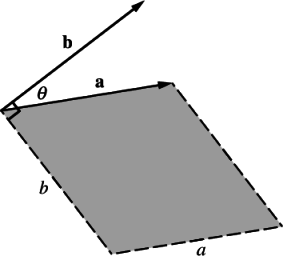
点积在不同坐标系下是不变的，因为它是由两个向量的大小和它们之间的角度所确定的。不变性的概念对连续介质力学很重要，在第4节中对坐标变换进行数学描述后，将进一步讨论。

1.3 两个向量的叉积

叉积（Cross product），又称向量积（Vector product）、叉乘。笛卡尔坐标系中，叉积\mathbf {a} \times \mathbf {b}的结果是与 \mathbf {a} 和\mathbf {b}都垂直的向量 \mathbf {c} 。其方向由右手定则决定，模长等于以两个向量为边的平行四边形的面积。

向量 \mathbf{a}=\left(a_{1}, a_{2}, a_{3}\right) 和向量\mathbf{b}=\left(b_{1}, b_{2}, b_{3}\right)的叉积定义如下:

\mathbf{a} \times \mathbf{b}=\left(a_{2} b_{3}-a_{3} b_{2}, a_{3} b_{1}-a_{1} b_{3}, a_{1} b_{2}-a_{2} b_{1}\right)=e_{i j k} a_{j} b_{k}

其中置换数e_{ijk}的定义如下：

e_{i j k}=\left{\begin{array}{ll}
0&\text { when any two indices are equal } \\
+1&\text { when } i, j, k \text { are an even permutation of } 1,2,3 \\
-1&\text { when } i, j, k \text { are an odd permutation of } 1,2,3
\end{array}\right.

其中偶数排列为123、231和312，奇数排列为132、213和321。叉积运算具有以下性质：

\begin{array}{c}
\mathbf{a} \times \mathbf{a}=\mathbf{0} \\
\mathbf{a} \times \mathbf{b}=-\mathbf{b} \times \mathbf{a} \\
\mathbf{a} \times(\mathbf{b}+\mathbf{c})=\mathbf{a} \times \mathbf{b}+\mathbf{a} \times \mathbf{c}
\end{array}

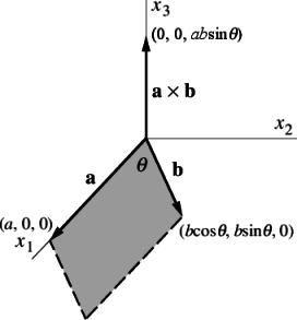
为了解释叉积的几何意义，定义两个位于笛卡尔坐标系 x_{1} x_{2} 平面上的两个向量 \mathbf{a} 和\mathbf{b} ，其中 \mathbf{a}=(a, 0,0) ，\mathbf{b}=(b \cos \theta, b \sin \theta, 0) . 则叉积 \mathbf{a} \times \mathbf{b}=(0,0, a b \sin \theta)是沿z轴的一个向量。因此，叉积代表一个法向量，其大小等于由向量定义的平行四边形\mathbf{a} 和\mathbf{b}的面积，方向与平行四边形所在平面垂直。法向量的方向遵循第4.1节中定义右手准则。

Figure 2: The vector product

1.4 两个向量的外积

两个向量\mathbf{a}和\mathbf{b}的外积，也被称为并向量积，结果是一个张量，运算不具有交换性的，由符号 \otimes表示：

\begin{aligned}
\mathbf{T}=\mathbf{a} \otimes \mathbf{b}=\mathbf{a b}^{T}&= \left[ \begin{array}{c} a_{x} \\ a_{y} \\ a_{z} \end{array} \right] \left[ \begin{array}{ccc} b_{x}&b_{y}& b_{z} \end{array} \right] \\ &=\left[\begin{array}{lll}
a_{x} b_{x}&a_{x} b_{y}&a_{x} b_{z} \\
a_{y} b_{x}&a_{y} b_{y}&a_{y} b_{z} \\
a_{z} b_{x}&a_{z} b_{y}&a_{z} b_{z}
\end{array}\right] .
\end{aligned}

在大多数文献中，我们会发现，为了简洁起见，向量的外积运算都忽略了并向量积运算符\otimes，简写为：

\mathbf{T}=\mathbf{a} \otimes \mathbf{b}=\mathbf{a b}

2. 二阶张量

二阶张量在这里被定义为一个线性向量函数，即它是一个将一个参数向量与另一个向量联系起来的函数。向量本身是一个一阶张量，标量是零阶张量。更高阶的张量将在后面简要讨论，但在大多数情况下，我们处理的是二阶张量，通常被简单地称为张量。

张量作为一个线性向量函数，其作用如下：

u_{i}=T_{i j} v_{j}

一个n-维的二阶张量T or T_{i j} 由n^{2} 个元素构成，可以用如下的对应于坐标轴x_{1}, x_{2}, \ldots, x_{n} 的标量数组来表示：

\mathbf{T}=T_{i j}=\left(\begin{array}{cccc}
T_{11}&T_{12}&\ldots&T_{1 n} \\
T_{21}&T_{22}&\ldots&T_{2 n} \\
\vdots&\vdots&\ddots&\vdots \\
T_{n 1}&T_{n 2}&\ldots&T_{n n}
\end{array}\right)

下标i=j的分量通常被称为对角分量，而那些i\neq j的分量则被称为非对角线分量。应该少用标量数组的方式表示张量，因为它可能会使运算变得不方便，而且对于2阶以上的张量来说，这种张量标记方式几乎变得无法使用。在本章的其余部分中，将使用具有9个分量的3维二阶张量来介绍张量的表示方法：

\mathbf{T}=T_{i j}=\left(\begin{array}{ccc}
T_{11}&T_{12}&T_{13} \\
T_{21}&T_{22}&T_{23} \\
T_{31}&T_{32}&T_{33}
\end{array}\right)

2.1 张量和向量的点积

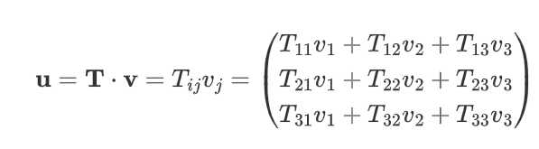
方程 u_i=T_{i j} v_j 可以用张量表示法写成一个点积运算，这个运算将一个几何向量转换为另一个几何向量（为方便起见，将向量都写成列向量）:

因此，一个向量 \mathbf{a} 和一个张量 \mathbf{T} 的内积产生一个向量 \mathbf{b}，如果该张量是非对称的，则该内积运算是不可交换的：

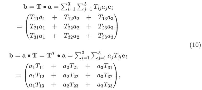
如果\mathbf{T}是对称张量，即：T_{ij}=T_{ji} ，则 \mathbf{a} \bullet \mathbf{T} = \mathbf{T} \bullet \mathbf{a} 。即对称张量与向量的内积是可交换的。

2.2 对称和反对称张量

如果一个张量的分量是对称的，即 \mathbf{T}=\mathbf{T}^{\mathrm{T}}，则称其为对称张量。反对称张量（skew or antisymmetric tensor）位于主对角线两侧对称的元素反号，即\mathbf{T}=-\mathbf{T}^{\mathrm{T}} ，这个定义意味着位于对角线上的元素T_{11}=T_{22}=T_{33}=0。 每一个二阶张量都可以用对称和反对称部分来表示，即：

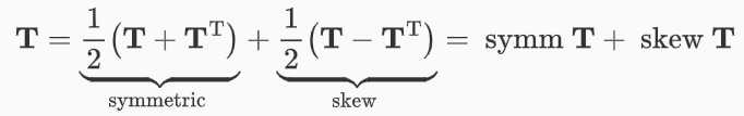
对称或反对称张量经坐标变换后仍会保持对称或反对称的性质，即对称性和反对称性是张量的内在属性，与它们所在的坐标系无关。

2.3 两个张量的标量积

两个张量的标量乘积用 \mathbf{T}: \mathbf{S} 表示，为二阶张量九个分量对应乘积之和：

\begin{aligned}
\mathbf{T}: \mathbf{S}=\sum_{i=1}^{3} \sum_{j=1}^{3} T_{i j} S_{i j} = \\
T_{i j} S_{i j}=& T_{11} S_{11}+T_{12} S_{12}+T_{13} S_{13}+\\
& T_{21} S_{21}+T_{22} S_{22}+T_{23} S_{23}+\\
& T_{31} S_{31}+T_{32} S_{32}+T_{33} S_{33}
\end{aligned}

也有一些作者用' : '符号来定义另一个标量积，在此表示为 \mathbf{T} \cdot \cdot \mathbf{\ S} ：

\begin{aligned}
\mathbf{T} \cdot \mathbf{S}=T_{i j} S_{j i}= \\
& T_{11} S_{11}+T_{12} S_{21}+T_{13} S_{31}+ \\
& T_{21} S_{12}+T_{22} S_{22}+T_{23} S_{32}+ \\
& T_{31} S_{13}+T_{32} S_{23}+T_{33} S_{33}
\end{aligned}

当然，对于任何一个对称的张量，没有必要区分这两个标量积的定义。

2.4 两个向量的张量积

The tensor product of two vectors, denoted by \mathbf{a b} (sometimes denoted \mathbf{a} \otimes \mathbf{b} ), is defined by the requirement that (\mathbf{a b}) \cdot \mathbf{v}=\mathbf{a}(\mathbf{b} \cdot \mathbf{v}) for all \mathbf{v} and produces a tensor whose components are evaluated as:

\mathbf{a b}=a_{i} b_{j}=\left(\begin{array}{ccc}
a_{1} b_{1}&a_{1} b_{2}&a_{1} b_{3} \\
a_{2} b_{1}&a_{2} b_{2}&a_{2} b_{3} \\
a_{3} b_{1}&a_{3} b_{2}&a_{3} b_{3}
\end{array}\right)

2.5 两个二阶张量的张量积

The tensor product of two tensors combines two operations \mathbf{T} and \mathbf{S} so that \mathbf{S} is performed first, i. e. (\mathbf{T} \cdot \mathbf{S}) \cdot \mathbf{v}=\mathbf{T} \cdot(\mathbf{S} \cdot \mathbf{v}) for all \mathbf{v} . It is denoted by (\mathbf{T} \cdot \mathbf{S}) and produces a tensor whose components are evaluated as:

P_{i j}=T_{i k} S_{k j}

The product is only commutative is both tensors are symmetric since

\mathbf{T} \cdot \mathbf{S}=\left[\mathbf{S}^{\mathrm{T}} \cdot \mathbf{T}^{\mathrm{T}}\right]^{\mathrm{T}}

2.6 张量的迹

张量的迹是张量的标量不变函数(scalar invariant function of the tensor)，其定义为：

\text {tr } \mathbf{T} = T_{ij} \delta_{ij} = T_{kk} = T_{11} + T_{22} + T_{22}

2.7 张量的行列式

The determinant of a tensor is also a scalar invariant function of the tensor denoted by

\begin{array}{c}
\operatorname{det} \mathbf{T}=\left|\begin{array}{ccc}
T_{11}&T_{12}&T_{13} \\
T_{21}&T_{22}&T_{23} \\
T_{31}&T_{32}&T_{33}
\end{array}\right|=\frac{1}{6} e_{i j k} e_{p q r} T_{i p} T_{j q} T_{k r}= \\
T_{11}\left(T_{22} T_{33}-T_{23} T_{32}\right)-T_{12}\left(T_{21} T_{33}-T_{23} T_{31}\right)+T_{13}\left(T_{21} T_{32}-T_{22} T_{31}\right)
\end{array}

3. 高阶张量

In Section [2.4](#2.4 两个向量的张量积) an operation was defined for the product of two vectors which produced a second rank tensor. Tensors of higher rank than two can be formed by the product of more than two vectors, e.g. a third rank tensor \mathbf{a b c} , a fourth rank tensor \mathbf{a b c d} . If one of the tensor products is replaced by a scalar (\cdot) product of two vectors, the resulting tensor is two ranks less than the original. For example, (\mathbf{a} \cdot \mathbf{b}) \mathbf{c d} is a second rank tensor since the product in brackets is a scalar quantity. Similarly if a scalar (\boldsymbol{:}) product of two tensors is substituted as in \mathbf{a b} \mathbf{~ : ~ c d} , the resulting tensor is four ranks less than the original. The process of reducing the rank of a tensor by a scalar product is known as contraction. The dot notation indicates the level of contraction and can be extended to tensors of any rank. In continuum mechanics tensors of rank greater than two are rare. The most common tensor operations to be found in continuum mechanics other than those in Sections 1 and 2 are:
a vector product of a vector \mathbf{a} and second rank tensor \mathbf{T} to produce a third rank tensor \mathbf{P}=\mathbf{a} \mathbf{T} whose components are:

P_{i j k}=a_{i} T_{j k}

a scalar product of a vector \mathbf{a} and third rank tensor \mathbf{P} to produce a second rank tensor \mathbf{T}=\mathbf{a} \cdot \mathbf{P} whose components are

T_{j k}=a_{i} P_{i j k}

a scalar (z) product of a fourth rank tensor \mathbf{C} and a second rank tensor \mathbf{S} to produce a second rank tensor \mathbf{T}=\mathbf{C}: \mathbf{S} whose components are

T_{i j}=C_{i j k l} S_{k l}

4 坐标系和坐标变换

连续介质力学中物理量的参考基础是我们工作的坐标系。如果坐标系发生转换，张量的分量就会发生变化。我们必须首先研究基坐标的性质，以确定坐标转换的规则。

4.1 笛卡尔坐标系

本文中我们只研究右手笛卡尔坐标系，其中的三个坐标轴，O_{x1}, O_{x2}和O_{x3}，相交于原点O且相互垂直。

Figure 3: 坐标系和方向余弦

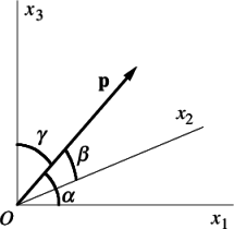
如图3所示，我们定义一个从原点出发的向量\mathbf{P}，与笛卡尔坐标系的x_{1}，x_{2}和x_3坐标轴的夹角分别为\alpha, \beta和\gamma。因此，向量\mathbf{P}的方向余弦定义为：cos \alpha, cos \beta和cos \gamma。方向余弦的大小可以表示为l_i=p_i/p，或者：

l = \frac{p}{|p|}

其中，p_i是指向量在相应坐标轴上的投影长度。

4.1 坐标旋转

考虑如图4所示的两组共原点的右手笛卡尔坐标系，分别标记为Ox_1x_2x_3和Ox^{'}_1x^{'}_2x^{'}_3：

Figure 4: 坐标旋转

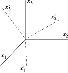
两个坐标系可以通过坐标轴的旋转而重合。 O x_{1}^{\prime} x_{2}^{\prime} x_{3}^{\prime} 相对于 O x_{1} x_{2} x_{3} 的方向余弦可以用来表示 O x_{1}^{\prime} x_{2}^{\prime} x_{3}^{\prime} 相对于O x_{1} x_{2} x_{3} 的位置： O x_{1}^{\prime} 相对于 O x_{1} x_{2} x_{3} 的方向余弦用 L_{11}, L_{12} 和L_{13} 表示 O x_{2}^{\prime} 和O x_{3}^{\prime} 相对于原坐标系的方向余弦则用L_{21}, L_{22}, L_{23} 和L_{31}, L_{32}, L_{33}表示。这个变换可以表示为：

\begin{array}{c|ccc}
O&x_{1}&x_{2}&x_{3} \\
\hline x_{1}^{\prime}&L_{11}&L_{12}&L_{13} \\
x_{2}^{\prime}&L_{21}&L_{22}&L_{23} \\
x_{3}^{\prime}&L_{31}&L_{32}&L_{33}
\end{array}

The matrix transformation can be expressed in a more compact form by defining the group of directional cosines as a tensor \mathbf{L}=L_{i i \cdot} . A coordinate \mathbf{x} in the O x_{1} x_{2} x_{3} axes can then be represented in the O x_{1}^{\prime} x_{2}^{\prime} x_{3}^{\prime} axes as:

\mathbf{x}^{\prime}=\mathbf{L} \cdot \mathbf{x}

Components of the transformation tensor \mathbf{L} must satisfy certain conditions since they are defined by two right-handed sets of axes. Since the axes are mutually perpendicular:

\begin{array}{l}
L_{11} L_{21}+L_{12} L_{22}+L_{13} L_{23}=0 \\
L_{21} L_{31}+L_{22} L_{32}+L_{23} L_{33}=0 \\
L_{31} L_{11}+L_{32} L_{12}+L_{33} L_{13}=0
\end{array}

and since the sums of squares of directional cosines are unity:

\begin{array}{l}
L_{11}^{2}+L_{12}^{2}+L_{13}^{2}=1 \\
L_{21}^{2}+L_{22}^{2}+L_{23}^{2}=1 \\
L_{31}^{2}+L_{32}^{2}+L_{33}^{2}=1
\end{array}

The two equations above describe the orthonormality conditions which can be expressed in a more compact form:

\mathbf{L} \cdot \mathbf{L}^{\mathbf{T}}=\mathbf{I}

The transformation matrix must satisfy one further requirement which ensures that both the sets of axes are right-handed. It is:

\operatorname{det} \mathbf{L}=1

5. 微分运算符

在向量标记法中，一个变量（标量、向量或张量）的空间导数是用Nabla算子\nabla表示的。它包含直角坐标系中对x、y和z的三个空间导数。

\nabla=\left(\begin{array}{l}
\frac{\partial}{\partial x} \\
\frac{\partial}{\partial y} \\
\frac{\partial}{\partial z}
\end{array}\right)=\left(\begin{array}{l}
\frac{\partial}{\partial x_{1}} \\
\frac{\partial}{\partial x_{2}} \\
\frac{\partial}{\partial x_{3}}
\end{array}\right)

5.1 梯度运算

• 一个标量的梯度结果是一个向量a，梯度运算也可以应用于高阶张量，它总是使张量升高一阶。

\operatorname{grad} \phi=\nabla \phi=\left(\begin{array}{l}
\frac{\partial \phi}{\partial x} \\
\frac{\partial \phi}{\partial y} \\
\frac{\partial \phi}{\partial z}
\end{array}\right) .

• 因此，对向量进行梯度运算则得到一个二阶张量：

\operatorname{grad} \mathbf{b}=\nabla \otimes \mathbf{b}=\left[\begin{array}{ccc}
\frac{\partial}{\partial x} b_{x}&\frac{\partial}{\partial x} b_{y}&\frac{\partial}{\partial x} b_{z} \
\frac{\partial}{\partial y} b_{x}&\frac{\partial}{\partial y} b_{y}&\frac{\partial}{\partial y} b_{z} \
\frac{\partial}{\partial z} b_{x}&\frac{\partial}{\partial z} b_{y}&\frac{\partial}{\partial z} b_{z}
\end{array}\right]

我们可以看到，这个操作是Nabla算子（一个特定的向量，见\nabla完整表达式）和一个任意向量b的外积，因此，它通常被写成：

\nabla \mathbf{b}

在本书中，我们使用式\operatorname{grad} \mathbf{b}所示的带有\otimes符号的完整表达方式。

5.2 散度运算

• 向量\mathbf{b}的散度是一个标量\phi，由Nabla算子和点运算符的组合表示，即\nabla \cdot ：

\operatorname{div} \mathbf{b}=\nabla \bullet \mathbf{b}=\sum_{i=1}^{3} \frac{\partial}{\partial x_{i}} b_{i}=\frac{\partial b_{1}}{\partial x_{1}}+\frac{\partial b_{2}}{\partial x_{2}}+\frac{\partial b_{3}}{\partial x_{3}}

• 一个二阶张量\mathbf{T}的散度是一个向量：

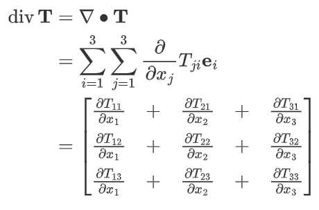
与梯度计算相反，散度运算的到的结果总是比原来的张量低一阶。因此，在标量上应用这个算子是没有意义的。

5.3 散度算子中的乘法规则

如果我们在散度项内有一个乘积，我们可以用乘积规则来分割这个项。根据散度内部的张量的阶数，我们必须应用不同的规则，现在对此进行介绍。

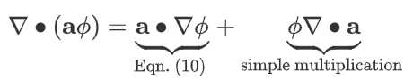
• 向量\mathbf{a}和标量\phi的乘积的散度可以按如下方式分割，结果是一个标量:

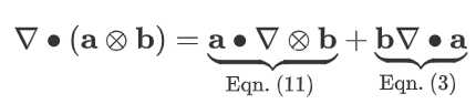
• 两个向量\mathbf{a}和\mathbf{b}的外积的散度可按如下方式分割，结果得到一个向量：

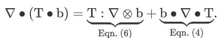
• 张量\mathbf{T}和向量\mathbf{b}的内积的散度可以按如下方式分割，结果是一个标量：

If one thinks that the product rule for the inner product of two vectors is missing, think about the result of the inner product of the two vectors and which tensor rank the result will have. After that, ask yourself how the divergence operator will change the rank.

1.3.1 The Total Derivative
The definition of the total derivative of an arbitrary quantity \phi - in the field of fluid dynamics is defined as:

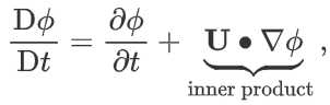
where \mathbf{U} represents the velocity vector. The last term in equation (1.22) denotes the inner product. Depending on the quantity \phi (scalar, vector, tensor, and so on), the correct mathematical expression for the second term on the right hand side (RHS) has to be applied. Example given:
- If \phi is a scalar, we have to use equation for inner product \mathbf{a} \cdot \mathbf{b} (Eq. 1),
- If \phi is a vector, we have to use equation for tensor inner product \mathbf{b}=\mathbf{T} \bullet \mathbf{a} (Eq. 10).

二 利用OpenFOAM进行张量计算²

OpenFOAM作为使用cpp编写的一个开源计算流体力学（Computational Fluid Dynamics, CFD）软件，其本身是架构在一系列基础数学运算库之上的，本质上是一个采用数值方法求解各类微分方程的cpp类库的集合。自然，我们也可以调用这些类库进行一些基础的数学运算，如本文所讲到的张量运算。

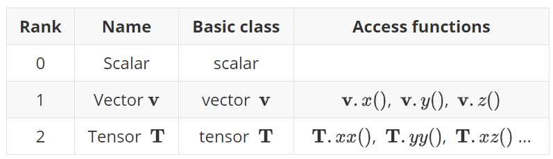
数学运算与OpenFOAM运算符

OpenFOAM中r=(0,1,2,3)。零阶张量称为标量（scalar),第一阶张量称为向量（Vector），第二阶张量（tensor），数学上称矩阵（Matrix）。二阶张量有9个分量，表示为T_{ij}，三阶张量有27个分量，表示为P_{ijk}。

取值运算表

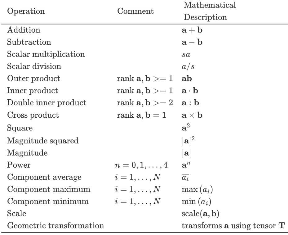
以下三个表格分别给出了张量运算在OpenFOAM编程中所使用的标记符号：

\text { Operations exclusive to tensors of rank } 2\\
\begin{array}{ccc}
\hline \text { Transpose }&\text { T }^{\text {T }}&\text { T.T() } \\
\text { Diagonal }&\operatorname{diag} \text { T }&\operatorname{diag}(\text { T }) \\
\text { Trace }&\operatorname{tr} \text { T }&\operatorname{tr}(\text { T) } \\
\text { Deviatoric component }&\operatorname{dev} \text { T }&\operatorname{dev}(\text { T) } \\
\text { Symmetric component }&\text { symm T }&\operatorname{symm}(\text { T }) \\
\text { Skew-symmetric component }&\text { skew T }&\operatorname{skew}(\text { T }) \\
\text { Determinant }&\operatorname{det} \text { T }&\operatorname{det}(\text { T) } \\
\text { Cofactors }&\operatorname{cof} \text { T }&\operatorname{cof}(\text { T) } \\
\text { Inverse }&\operatorname{inv} \text { T }&\operatorname{inv}(\text { T }) \\
\text { Hodge dual }&* \text { T }&* \text { T } \\
\hline
\end{array}

\begin{array}{ccc}
\text { Operations exclusive to scalars } \\
\hline
\text { Sign (boolean) }&\operatorname{sgn}(s)&\operatorname{sign}(\mathrm{s}) \\
\text { Positive (boolean) }&s>=0&\operatorname{pos}(\mathrm{s}) \\
\text { Negative (boolean) }&s<0&\operatorname{neg}(\mathrm{s}) \\
\text { Limit }&n \text { scalar }&\operatorname{limit}(s, n)&\operatorname{limit}(\mathrm{s}, \mathrm{n}) \\
\text { Square root }&\sqrt{s}&\operatorname{sqrt}(\mathrm{s}) \\
\text { Exponential }&\exp s&\exp (\mathrm{s}) \\
\text { Natural logarithm }&\ln s&\log (\mathrm{s}) \\
\text { Base } 10 \text { logarithm }&\log _{10} s&\log 10(\mathrm{~s}) \\
\text { Sine }&\sin s&\sin (\mathrm{s}) \\
\text { Cosine }&\cos s&\cos (\mathrm{s}) \\
\text { Tangent }&\tan s&\tan (\mathrm{s}) \\
\text { Arc sine }&\operatorname{asin} s&\operatorname{asin}(\mathrm{s}) \\
\text { Arc cosine }&\operatorname{acos} s&\operatorname{acos}(\mathrm{s}) \\
\text { Arc tangent }&\operatorname{atan} s&\operatorname{atan}(\mathrm{s}) \\
\text { Hyperbolic sine }&\sinh s&\sinh (\mathrm{s}) \\
\text { Hyperbolic cosine }&\cosh s&\cosh (\mathrm{s}) \\
\text { Hyperbolic tangent }&\tanh s&\tanh (\mathrm{s}) \\
\text { Hyperbolic arc sine }&\operatorname{asinh} s&\operatorname{asinh}(\mathrm{s}) \\
\text { Hyperbolic arc cosine }&\operatorname{acosh} s&\operatorname{acosh}(\mathrm{s}) \\
\text { Hyperbolic arc tangent }&\operatorname{atanh} s&\operatorname{atanh}(\mathrm{s}) \\
\text { Error function }&\operatorname{erf} s&\operatorname{erf}(\mathrm{s}) \\
\text { Complement error function }&\operatorname{erfc} s&\operatorname{erf}(\mathrm{s}) \\ \hline
\end{array}

编程案例

OpenFOAM的数学运算库中，用于零阶、一阶和二阶张量计算的库有 tensor 和 symmTensor 等。OpenFOAM 有一个现成的张量计算的例子，位置是 $FOAM_APP/test/tensor。我们拆开来说明下。

1. 定义二阶张量

以下代码定义了二阶张量t_1和t_2，并读取了其行向量和单个元素，最终输出到terminal。

#include "tensor.H"
#include "IOstreams.H"
using namespace Foam;
int main()
{
    /* 定义二阶张量 */
    tensor t1(1E-1, 2E-1, 3E-1, 4E-1, 5E-1, 6E-1, 7E-1, 8E-1, 9E-1);
    tensor t2(1E-1, 2E-1, 3E-1, 1E-1, 2E-1, 3E-1, 1E-1, 2E-1, 3E-1);

    /* 读取二阶张量的行向量 */
    Info<< t1.x() << t1.y() << t1.z() << endl;

    /* 读取二阶张量行向量的元素 */
    Info<< t1.x().x() << "  " << t1.x().y() << "  "  << t1.x().z() << endl;
    Info<< t1.y().x() << "  "  << t1.y().y() << "  " << t1.y().z() << endl;
    Info<< t1.z().x()  << "  " << t1.x().y() << "  " << t1.z().z() << endl;

    /* 或者采用双下标 */
    Info<< t1.xx() << "  " << t1.xy() << "  "  << t1.xz() << endl;
    Info<< t1.yx() << "  "  << t1.yy() << "  " << t1.yz() << endl;
    Info<< t1.zx()  << "  " << t1.zy() << "  " << t1.zz() << endl;
    return 0;
}

2. 二阶张量求和差

#include "tensor.H"
#include "IOstreams.H"
using namespace Foam;
int main()
{
    /* 定义二阶张量 */
    tensor t1(1E-1, 2E-1, 3E-1, 4E-1, 5E-1, 6E-1, 7E-1, 8E-1, 9E-1);
    tensor t2(1E-1, 2E-1, 3E-1, 1E-1, 2E-1, 3E-1, 1E-1, 2E-1, 3E-1);

    /* 求和：对应元素相加 */
    tensor t3 = t1 + t2;
    /* 求差：对应元素相减 */
    tensor t5 = t1 - t2;
    Info<< "Tensor t5: " << t5 << endl;

    return 0;
}

3. 二阶张量求逆

#include "tensor.H"
#include "IOstreams.H"
using namespace Foam;
int main()
{
    tensor t4(3,-2,1,-2,2,0,1, 0, 4);

    Info<< "The inverse of tensor t4 is: " <<inv(t4) << endl;  // 求逆运算
    return 0;
}

其中inv() 是二阶张量的求逆（inverse）函数。

4. 特征值、特征向量与行列式

对于一个固定的矩阵A，一般的向量被他transform之后都会改变方向，但是有一些特殊的向量，被A映射了之后还是保持它本来的方向，改变的只是它的模长。这些特殊向量的方向不变性表达出来就是这样的：
A \mathbf{v}=\lambda \mathbf{v}
where:
A = a diagonalizable square matrix of dimension m-by-m;
v = a (non-zero) vector of dimension m (right eigenvector);
λ = a scalar corresponding to v (eigenvalue) ;

等式的右边，\mathbf{v}表示向量原本的方向，\lambda表示向量模长的变化。特征向量的定义就是这些特殊的向量。使用特征向量和特征值的概念可以简化矩阵的幂运算，即：如果使用矩阵A对向量\mathbf{v}做100次变换：
A^{100} \mathbf{v} = \lambda ^{100} \mathbf{v} \nonumber
将原来的矩阵的乘法转换为了标量的乘法。另外，矩阵的迹（trace）定义为主对角线上的元素之和。

#include "tensor.H"
#include "IOstreams.H"
using namespace Foam;
int main()
{
    tensor t6(1,0,-4,0,5,4,-4,4,3);

    Info<< "tensor " << t6 << endl;
    vector e = eigenValues(t6);      // 特征值
    Info<< "eigenvalues " << e << endl;

    tensor ev = eigenVectors(t6);    // 特征向量
    Info<< "eigenvectors " << ev << endl;

    scalar tr_ = tr(t6);    // 矩阵的迹
    Info<< "Trace = " << tr_ << endl;

    // 矩阵行列式的值等于特征值的积
    Info<< "Check determinant " << e.x()*e.y()*e.z() << "<-- 特征值的乘积 = 行列式的值--> " << det(t6) << endl;

    vector v1(1,2,3);
    vector v2(4,5,6);
    vector v6 = v1^v2;   // ^表示叉积,只在一阶张量间使用.
    Info << "v6" << v6 << endl;

    return 0;
}

对于以下代码尚未完全理解~??

    Info<< "Check eigenvectors "
        << (eigenVectors(t6, e) & t6) << " "
        << (e.x()*eigenVectors(t6, e).x())
        << (e.y()*eigenVectors(t6, e).y())
        << (e.z()*eigenVectors(t6, e).z())
        << endl;

因为二阶张量t_6设置为对称矩阵，因此可以使用一些特殊的函数：

    tensor t6(1,0,-4,0,5,4,-4,4,3);
    symmTensor t7(1, 0, -4, 5, 4, 3);

    Info<< "Check eigenvalues for symmTensor "
        << eigenValues(symm(t6)) - eigenValues(tensor(symm(t6))) << endl;

以上代码中，symm(t6)的返回值是(1 0 -4 5 4 3)，即对称阵的上三角部分。运行上述代码，你应该能得到如下返回值：

 t6 - t7 = (0 0 0 0 0 0 0 0 0)
Check eigenvalues for symmTensor (0 0 0)
(1 0 -4 5 4 3)
(1 0 -4 0 5 4 -4 4 3)

可见，对于对称阵，采用上述t6和t7两种方式声明和定义均可，是等价的。以下代码展示了三维二阶张量内积的计算：

    tensor t1(
    1, 2, 3, 
    4, 5, 6, 
    7, 8, 9);
    tensor t7(
    1, 2, 3, 
    2, 4, 5, 
    3, 5, 6);
    Info<< "Check transformation "
        << (t1 & t7)  // 张量运算尽可能用括号括起来
        << " 张量内积（矩阵乘法）  " << endl;
    Info<< (t1 & t7 & t1.T()) 
        << endl;

此外，OpenFOAM 还提供了专门处理对称矩阵的库 symmTensor，详见 $FOAM_APP/test/tensor/Test_tensor.C。

5. 构造对称张量

上一节给出了使用symmTensor t7(1, 0, -4, 5, 4, 3);方式定义对称二阶张量。下面我们将研究其他构造对称张量的方式。

    symmTensor st1(1, 2, 3, 4, 5, 6);
    symmTensor st2(7, 8, 9, 10, 11, 12);


    Info<< "Check dot product of symmetric tensors "
        << (st1 & st2) << endl;

    Info<< "Check inner sqr of a symmetric tensor "  // 相等
        << innerSqr(st1) << " " << innerSqr(st1) - (st1 & st1) << endl;

下面的代码中，twoSymm(T)将二阶张量的主对角线元素翻倍，沿主对角线对称的元素相加构成一个对称张量：

\begin{aligned}
{\rm twoSymm}(\boldsymbol{T}) &\equiv& \boldsymbol{T} + \boldsymbol{T}^T \\
&=& \left(
\begin{aligned}
2T_{11}&T_{12} + T_{21}&T_{13} + T_{31} \\
T_{21} + T_{12}&2T_{22}&T_{23} + T_{32} \\
T_{31} + T_{13}&T_{32} + T_{23}&2T_{33}
\end{aligned} \right)
\end{aligned}

这一命令是使用以下代码实现的：

Definition: src/OpenFOAM/primitives/Tensor/TensorI.H

//- Return twice the symmetric part of a tensor
template<class Cmpt>
inline SymmTensor<Cmpt> twoSymm(const Tensor<Cmpt>& t)
{
    return SymmTensor<Cmpt>
    (
        2*t.xx(), (t.xy() + t.yx()), (t.xz() + t.zx()),
                  2*t.yy(),          (t.yz() + t.zy()),
                                     2*t.zz()
    );
}

因此，运行以下代码：

    symmTensor st1(1, 2, 3, 4, 5, 6);
    symmTensor st2(7, 8, 9, 10, 11, 12);

    Info<< "Twice the Symmetric Part of a Second Rank Tensor"
        << twoSymm(st1&st2) << endl;

    Info<< "Check symmetric part of dot product of symmetric tensors "
        << twoSymm(st1&st2) - ((st1&st2) + (st2&st1)) << endl;

你应该能得到以下输出：

Twice the Symmetric Part of a Second Rank Tensor(100 152 182 222 262 308)
Check symmetric part of dot product of symmetric tensors (0 0 0 0 0 0 0 0 0)

另一个可以用来构造二阶对称张量的命令是symm(T)，它所构造的张量元素分量正好是twoSymm(T)构造的对称张量的一半：
\begin{aligned}
{\rm symm}(\boldsymbol{T}) &\equiv& \frac{1}{2} (\boldsymbol{T} + \boldsymbol{T}^T) \\
&=& \frac{1}{2} \left(
\begin{matrix}
2T_{11}&T_{12} + T_{21}&T_{13} + T_{31} \\
T_{21} + T_{12}&2T_{22}&T_{23} + T_{32} \\
T_{31} + T_{13}&T_{32} + T_{23}&2T_{33}
\end{matrix} \right)
\end{aligned}

这一命令是由以下代码实现的：

Definition: src/OpenFOAM/primitives/Tensor/TensorI.H

//- Return the symmetric part of a tensor
template<class Cmpt>
inline SymmTensor<Cmpt> symm(const Tensor<Cmpt>& t)
{
    return SymmTensor<Cmpt>
    (
        t.xx(), 0.5*(t.xy() + t.yx()), 0.5*(t.xz() + t.zx()),
                t.yy(),                0.5*(t.yz() + t.zy()),
                                       t.zz()
    );
}

通过给定张量构造反对称张量则可以使用skew(T):

\begin{aligned}
{\rm skew}(\boldsymbol{T}) &\equiv& \frac{1}{2} (\boldsymbol{T} – \boldsymbol{T}^T) \\
&=& \frac{1}{2} \left(
\begin{matrix}
0&T_{12} – T_{21}&T_{13} – T_{31} \\
T_{21} – T_{12}&0&T_{23} – T_{32} \\
T_{31} – T_{13}&T_{32} – T_{23}&0
\end{matrix} \right)
\end{aligned}

Definition: src/OpenFOAM/primitives/Tensor/TensorI.H

//- Return the skew-symmetric part of a tensor
template<class Cmpt>
inline Tensor<Cmpt> skew(const Tensor<Cmpt>& t)
{
    return Tensor<Cmpt>
    (
        0.0, 0.5*(t.xy() - t.yx()), 0.5*(t.xz() - t.zx()),
        0.5*(t.yx() - t.xy()), 0.0, 0.5*(t.yz() - t.zy()),
        0.5*(t.zx() - t.xz()), 0.5*(t.zy() - t.yz()), 0.0
    );
}

速度梯度张量场的symm（对称）和skew（反对称）操作经常出现在源代码中。下面是一个典型的例子。

Usage Example: src/TurbulenceModels/turbulenceModels/RAS/SSG/SSG.C

    tmp<volTensorField> tgradU(fvc::grad(U));
    const volTensorField& gradU = tgradU();

    volSymmTensorField b(dev(R)/(2*k_));
    volSymmTensorField S(symm(gradU));
    volTensorField Omega(skew(gradU));

In the above code, the symmetric and antisymmetric parts of the velocity gradient tensor \frac{∂u_j}{∂x_i} are defined as follows:

\begin{aligned}
S_{ij} &=& \frac{1}{2} \left( \frac{\partial u_j}{\partial x_i} + \frac{\partial u_i}{\partial x_j} \right), \\
\Omega_{ij} &=& \frac{1}{2} \left( \frac{\partial u_j}{\partial x_i} – \frac{\partial u_i}{\partial x_j} \right),
\end{aligned}

where S_{ij} is the strain rate tensor and \Omega_{ij} is the vorticity (spin) tensor.

6 其他待完善

    symmTensor st1(1, 2, 3, 4, 5, 6);
    symmTensor st2(7, 8, 9, 10, 11, 12);

    tensor t1(1, 2, 3, 4, 5, 6, 7, 8, 9);
    tensor t6(1,0,-4,0,5,4,-4,4,3);
    tensor t7(1, 2, 3, 2, 4, 5, 3, 5, 6);
    vector v1(1, 2, 3);

    Info<< sqr(v1) << endl;
    Info<< symm(t7) << endl;
    Info<< twoSymm(t7) << endl;
    Info<< magSqr(st1) << endl;
    Info<< mag(st1) << endl;

Reference

[1] 用 OpenFOAM 进行张量计算 - 知乎

[2] Tensor Operations in OpenFOAM | CFD WITH A MISSION

[3] Tensor Mathematics | CFD Direct | Architects of OpenFOAM

[4] High-level programming in OpenFOAM