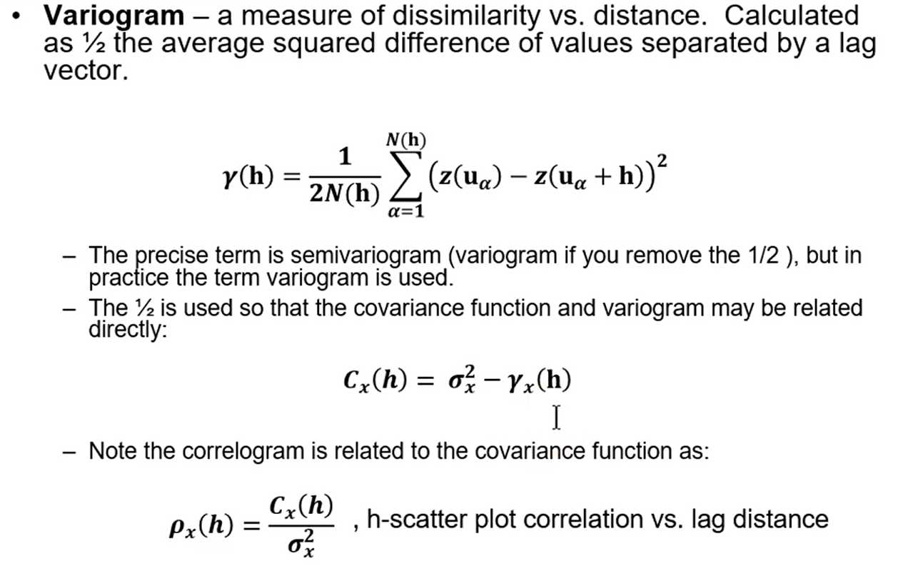
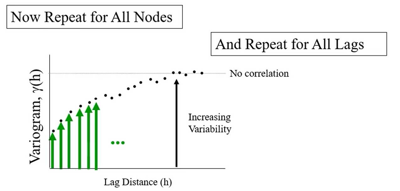
Recall: Variogram
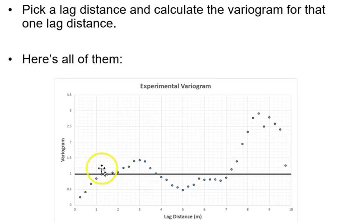
An example
Example data and calculation process can be download from:
Semivariogram_1D_Porosity.xlsx
The variogram, covariance function and correlation coefficient are equivalent tools for characterizing spatial two-point correlation (assuming stationarity):
$$
\begin{aligned}
\gamma_{x}(\mathbf{h}) &=\boldsymbol{\sigma}{x}^{2}-\boldsymbol{C}{x}(\boldsymbol{h}) \\
&=\boldsymbol{\sigma}{x}^{2}\left(1-\boldsymbol{\rho}{x}(\boldsymbol{h})\right) \quad \rho_{x}(\boldsymbol{h})=\frac{\boldsymbol{C}{x}(\boldsymbol{h})}{\sigma{x}^{2}}
\end{aligned}
$$
where:
$$
\begin{array}{r}
\boldsymbol{C}{x}(\mathbf{h})=\boldsymbol{E}{\boldsymbol{X}[\mathbf{u}) \cdot \boldsymbol{X}(\mathbf{u}+\mathbf{h})}-[\boldsymbol{E}{\boldsymbol{X}(\mathbf{u})} \cdot \boldsymbol{E}{\boldsymbol{X}(\mathbf{u}+\mathbf{h})}], \forall \mathbf{u}, \mathbf{u}+\mathbf{h} \in \boldsymbol{A} \\
C{x}(0)=\sigma_{x}^{2}
\end{array}
$$
$$
\boldsymbol{C}{x}(\mathbf{h}) = \frac{ \sum{\alpha=1}^{n} x \left( \mathbf{u} _ {\alpha} \right) \cdot x\left(\mathbf{u}_{\alpha}+\mathbf{h}\right)}{n}-(\bar{x})^{2}
$$
if stationary mean.
Stationarity entails that:
$$
\begin{gathered}
m(\mathbf{u})=m(\mathbf{u}+\mathbf{h})=m=E{Z}, \forall \mathbf{u} \in A \\
\operatorname{Var}(\mathbf{u})=\operatorname{Var}(\mathbf{u}+\mathbf{h})=\sigma^{2}=\operatorname{Var}{Z}, \forall \mathbf{u} \in A
\end{gathered}
$$
- Covariance Function - a measure of similarity vs. distance. Calculated as the average product of values separated by a lag vector centered by the square of the mean.
$$
\boldsymbol{C}{x}(\mathbf{h})=\frac{\sum{\alpha=1}^{n} x\left(\mathbf{u}{\alpha}\right) \cdot x\left(\mathbf{u}{\alpha}+\mathrm{h}\right)}{n}-(\bar{x})^{2}, \text { if stationary mean }
$$
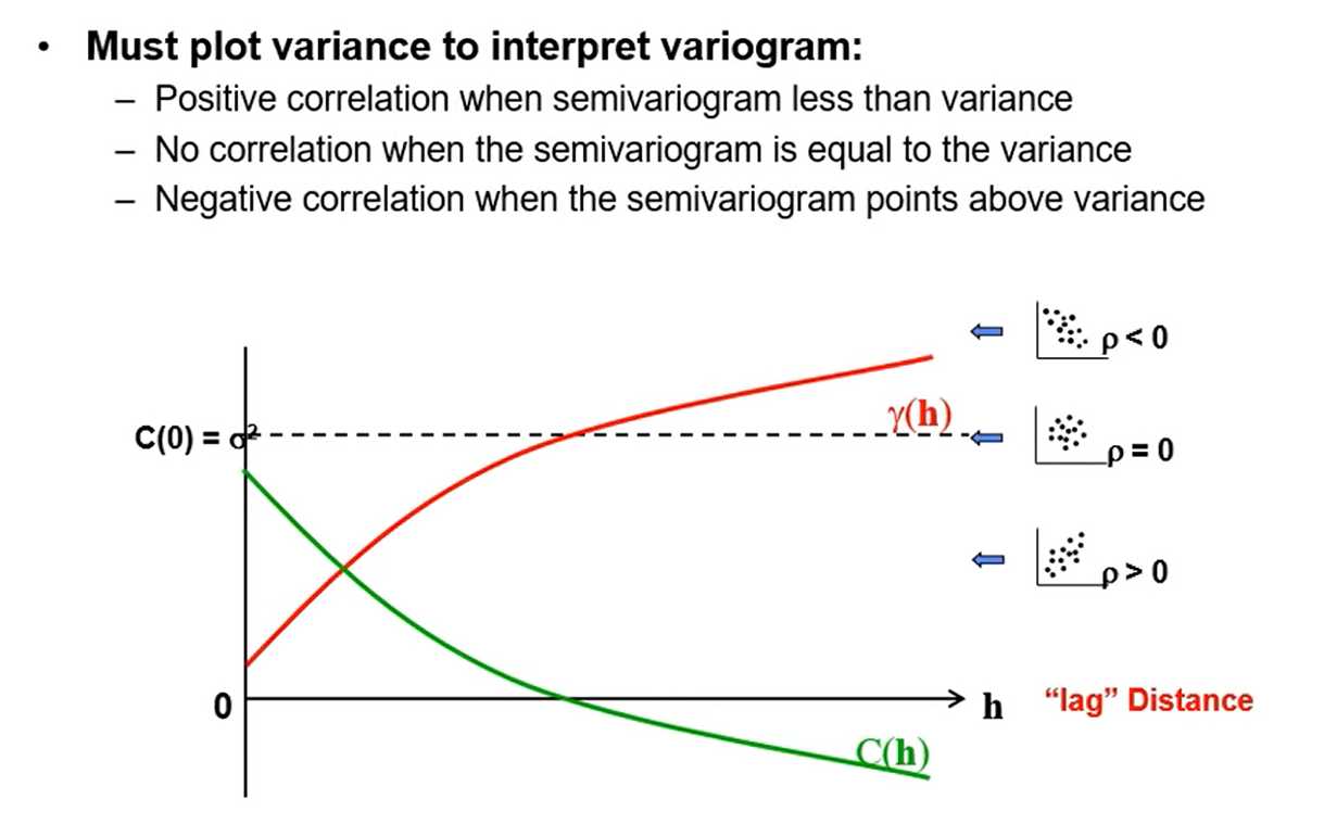
- The covariance function is the variogram upside down. $\gamma_{x}(\mathbf{h})=\sigma_{x}^{2}-C_{x}(\boldsymbol{h})$
- We model variograms, but inside the kriging and simulation methods they are converted to covariance values for numerical convenience.
Spoiler alert
We need to practically calculate and model spatial continuity. From
the available and often sparse subsurface data.
1. Calculate variogram with irregularly spaced data
— Search templates with parameters
2. Valid spatial model
— Fit with a couple different, nest (additive) spatial continuity models
e.g. nugget, spherical, exponential and Gaussian
3. Full 3D spatial continuity model
— Model primary directiqs, i.e. major horizontal, minor horizontal and
vertical and combine together with assumption of geometric
anisotropy
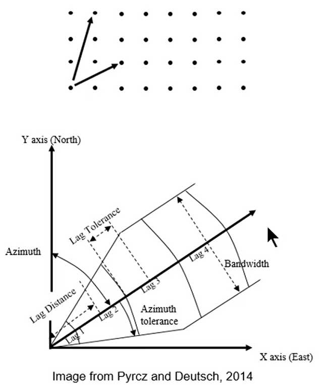
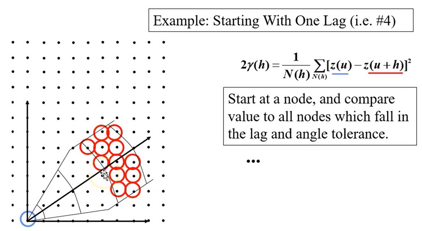
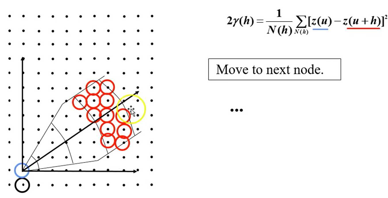
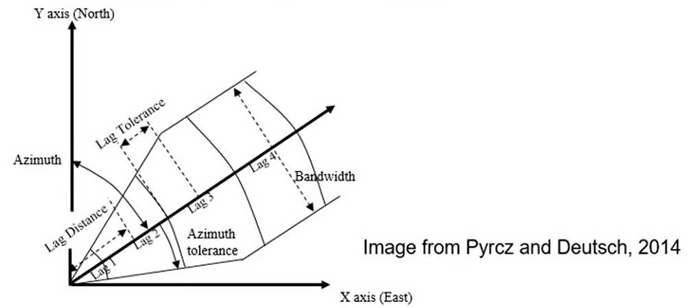
How do we get pairs separated by lag vector?
- Regular spaced data:
- Specify as offsets of grid units
- Fast calculation
- Diagonal directions are awkward
- Irregular spaced data:
- Nominal distance for each lag
- Distance tolerance
- Azimuth direction
- Azimuth tolerance
- Dip direction
- Dip tolerance
- Bandwidth (maximum deviation) in originally horizontal plane
- Bandwidth in originally vertical plane
• Data transformation:
— Transform a continuous variable to a Gaussian or normal distribution, for use with / consistency with Gaussian simulation methods
— Transform a categorical variable to a series of indicator variables for indicator methods and categorical to continuous for truncated Gaussian methods
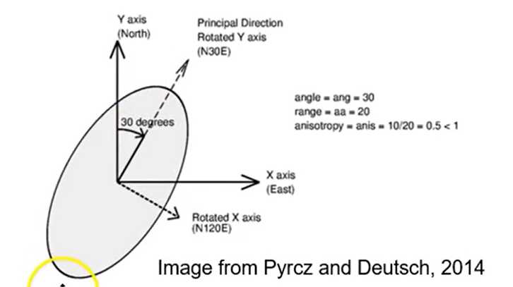
• Coordinate transformation:
— Variograms are calculated ali6ned with the stratigraphic framework
— Otherwise the spatial continuity will be underestimated
• Should calculate the variogram on the variable being modeled with transforms (data and coordinates)
• Calculate the variogram, as this is what we model and apply in estimation and simulation (more later).
Chossing the directions
• Inspect the data and interpretations, sections, plan views, ...
• Azimuth angles in degrees clockwise from north
• Review multiple directions before choosing a set of perpendicular directions
- Omnidirectional: all directions taken together —› often yields the most well-behaved variograms.
- Major horizontal direction & two perpendicular to major direction
- All anisotropy in geostatistics is geometric
— three mutually orthogonal directions with ellipsoidal change in the other directions:
Guidance for Variogram Calculation Parameters:
• Lag separation distance should coincide with data spacing
• Lag tolerance typically chosen to be 1/2 lag separation distance
— in cases of erratic variograms, may choose to overlap calculations so lag tolerance > 1/2 lag separation, results in more pairs.
• The variogram is only valid for a distance one half of the field size: start leaving data out of calculations with larger distances
Comments NOTHING