一维信号的滤波器效果对比

Please refresh the page if equations are not rendered correctly.
---------------------------------------------------------------

1. 实现代码与结果对比

import numpy as np
import matplotlib.pyplot as plt
from scipy.signal import savgol_filter, medfilt
import scipy.fftpack
import polykriging as pk


def savitzky_golay(y, window_size, order, deriv=0, rate=1):
    """
    Smooth (and optionally differentiate) data with a Savitzky-Golay filter.
    The Savitzky-Golay filter removes high frequency noise from data.
    It has the advantage of preserving the original shape and
    features of the signal better than other types of filtering
    approaches, such as moving averages techniques.

    [Cookbook/SavitzkyGolay - SciPy wiki dump](https://scipy.github.io/old-wiki/pages/Cookbook/SavitzkyGolay)
    [Savitzky-Golay滤波器 推导整理 - 知乎](https://zhuanlan.zhihu.com/p/535913266)

    Parameters
    ----------
    y : array_like, shape (N)
        the values of the time history of the signal.
    window_size : int
        the length of the window. Must be an odd integer number.
    order : int
        the order of the polynomial used in the filtering.
        Must be less then `window_size` - 1.
    deriv: int
        the order of the derivative to compute (default = 0 means only smoothing)
    Returns
    -------
    ys : ndarray, shape (N)
        the smoothed signal (or it's n-th derivative).
    Notes
    -----
    The Savitzky-Golay is a type of low-pass filter, particularly
    suited for smoothing noisy data. The main idea behind this
    approach is to make for each point a least-square fit with a
    polynomial of high order over a odd-sized window centered at
    the point.
    Examples
    --------
    t = np.linspace(-4, 4, 500)
    y = np.exp( -t**2 ) + np.random.normal(0, 0.05, t.shape)
    ysg = savitzky_golay(y, window_size=31, order=4)
    import matplotlib.pyplot as plt
    plt.plot(t, y, label='Noisy signal')
    plt.plot(t, np.exp(-t**2), 'k', lw=1.5, label='Original signal')
    plt.plot(t, ysg, 'r', label='Filtered signal')
    plt.legend()
    plt.show()
    References
    ----------
    .. [1] A. Savitzky, M. J. E. Golay, Smoothing and Differentiation of
       Data by Simplified Least Squares Procedures. Analytical
       Chemistry, 1964, 36 (8), pp 1627-1639.
    .. [2] Numerical Recipes 3rd Edition: The Art of Scientific Computing
       W.H. Press, S.A. Teukolsky, W.T. Vetterling, B.P. Flannery
       Cambridge University Press ISBN-13: 9780521880688
    """
    import numpy as np
    from math import factorial

    try:
        window_size = np.abs(int(window_size))
        order = np.abs(int(order))
    except ValueError:
        raise ValueError("window_size and order have to be of type int")
    if window_size % 2 != 1 or window_size < 1:
        raise TypeError("window_size size must be a positive odd number")
    if window_size < order + 2:
        raise TypeError("window_size is too small for the polynomials order")
    order_range = range(order + 1)
    half_window = (window_size - 1) // 2
    # precompute coefficients
    b = np.mat([[k ** i for i in order_range] for k in range(-half_window, half_window + 1)])
    # `.A` means convert matrix to array
    m = np.linalg.pinv(b).A[deriv] * rate ** deriv * factorial(deriv)
    # pad the signal at the extremes with
    # values taken from the signal itself
    first_vals = y[0] - np.abs(y[1:half_window + 1][::-1] - y[0])
    last_vals = y[-1] + np.abs(y[-half_window - 1:-1][::-1] - y[-1])
    y = np.concatenate((first_vals, y, last_vals))
    return np.convolve(m[::-1], y, mode='valid')


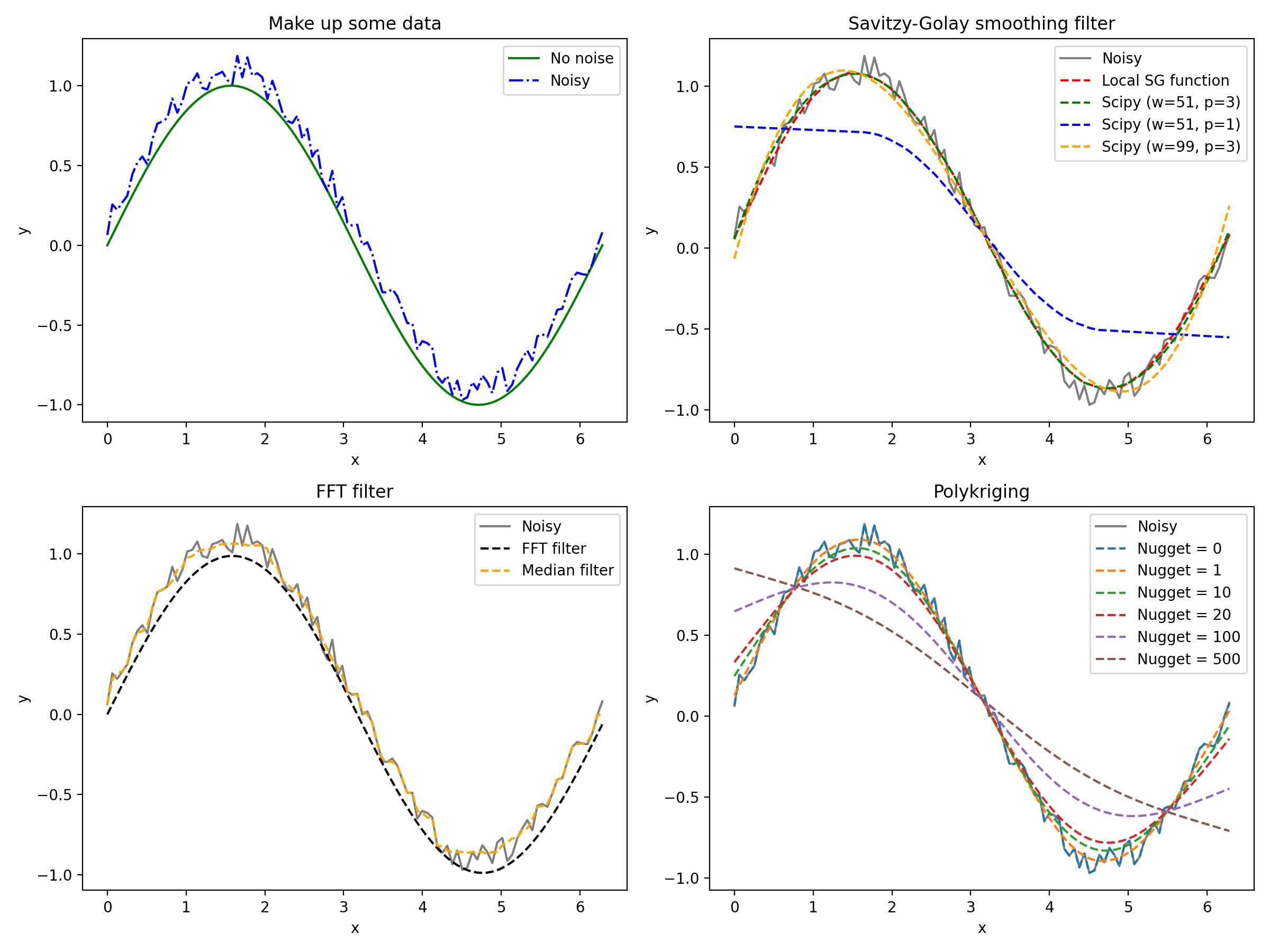
if __name__ == '__main__':
    """ Locally defined Savitzky-Golay filter """
    N = 100
    x = np.linspace(0, 2 * np.pi, N)
    y = np.sin(x) + np.random.random(N) * 0.2

    fig = plt.figure(figsize=(12, 9), dpi=200)
    ax = fig.add_subplot(221)
    # distance between two adjacent rows of subplots.
    fig.subplots_adjust(hspace=0.3, wspace=0.3)

    # ax.set_title('Savitzy-Golay smoothing filter')
    ax.plot(x, np.sin(x), color='green', label='No noise', linestyle='-')
    ax.plot(x, y, color='blue', label='Noisy', linestyle='-.')
    ax.legend(loc='best')
    ax.set_xlabel('x')
    ax.set_ylabel('y')
    ax.set_title('Make up some data')

    """ Savitzky-Golay filter """
    ax2 = fig.add_subplot(222)
    yhat_scipy = savgol_filter(y, 51, 3)  # window size 51, polynomial order 3
    yhat_scipy_2 = savgol_filter(y, 51, 1)  # window size 51, polynomial order 3
    yhat_scipy_3 = savgol_filter(y, 99, 3)  # window size 51, polynomial order 3
    yhat = savitzky_golay(y, 51, 3)  # window size 51, polynomial order 3
    ax2.plot(x, y, color='gray', label='Noisy', linestyle='-')
    ax2.plot(x, yhat, color='red', label='Local SG function', linestyle='--')
    ax2.plot(x, yhat_scipy, color='green', linestyle='--', label='Scipy (w=51, p=3)')
    ax2.plot(x, yhat_scipy_2, color='blue', linestyle='--', label='Scipy (w=51, p=1)')
    ax2.plot(x, yhat_scipy_3, color='orange', linestyle='--', label='Scipy (w=99, p=3)')
    ax2.legend(loc='best')
    ax2.set_xlabel('x')
    ax2.set_ylabel('y')
    ax2.set_title('Savitzy-Golay smoothing filter')

    """ FFT """
    # scipy.fftpack.rfft is a fast version of scipy.fftpack.fft for real inputs.
    w = scipy.fftpack.rfft(y)
    # DFT sample frequencies (for usage with rfft, irfft).
    f = scipy.fftpack.rfftfreq(N, x[1] - x[0])
    # If our original signal time was in seconds, this is now in Hz
    spectrum = w ** 2

    # High-pass filter
    cutoff_idx = spectrum < (spectrum.max() / 10)
    w2 = w.copy()
    w2[cutoff_idx] = 0

    ax3 = fig.add_subplot(223)
    y2 = scipy.fftpack.irfft(w2)
    ax3.plot(x, y, color='gray', label='Noisy', linestyle='-')
    ax3.plot(x, y2, color='black', linestyle='--', label='FFT filter')

    """ Median filter """
    y3 = medfilt(y, 11)
    ax3.plot(x, y3, color='orange', linestyle='--', label='Median filter')

    ax3.legend(loc='best')
    ax3.set_xlabel('x')
    ax3.set_ylabel('y')
    ax3.set_title('FFT filter')

    """ Polykriging """
    data_set = np.hstack((x.reshape(-1,1),y.reshape(-1,1)))

    name_drift, name_cov = 'lin', 'cub'
    nuggetEffect = [0, 1, 10, 20, 100, 500]

    ax4 = fig.add_subplot(224)
    ax4.plot(x, y, color='gray', label='Noisy', linestyle='-')
    for ng in nuggetEffect:
        # Kriging model and prediction with mean, Kriging expression
        # and the corresponding standard deviation as output.
        mean_prediction, expr, std_prediction = pk.kriging.curve2D.curve2Dinter(
            data_set, name_drift, name_cov,
            nuggetEffect=ng, interp=x, return_std=True)
        ax4.plot(x, mean_prediction, label='Nugget = ' + str(ng), linestyle='--')
    ax4.legend(loc='best')
    ax4.set_xlabel('x')
    ax4.set_ylabel('y')
    ax4.set_title('Polykriging')
    plt.tight_layout()
    plt.show()

2. 滤波器的特点

以下内容由Chat-GPT 3.5生成：

Comparing Smoothing Filters for Curves: Kriging, Savitzky-Golay (SG) Filter, Fast Fourier Transform, and Median Filter

1. Kriging:
   • Mathematical Basis: Kriging is a geostatistical interpolation method based on spatial correlation models. It estimates curve values by considering the weighted average of neighboring data points, with weights determined by variogram models.
   • Use Case: Kriging is effective for smoothing curves when the underlying data exhibit spatial correlation or when you want to capture spatial trends in the curve.
   • Pros: Handles irregularly spaced data well, incorporates spatial correlation, provides uncertainty estimates.
   • Cons: Computationally intensive, may require variogram modeling, not suitable for all curve types.
2. Savitzky-Golay (SG) Filter:
   • Mathematical Basis: SG filter is a polynomial smoothing technique that fits a polynomial to a moving window of data points and uses the polynomial coefficients to estimate smoothed values.
   • Use Case: SG filtering is excellent for removing noise from curves with well-defined peaks and valleys.
   • Pros: Preserves the shape of the underlying curve, computationally efficient, versatile.
   • Cons: Not suitable for all types of noise or curves, window size and polynomial degree selection can impact results.
3. Fast Fourier Transform (FFT):
   • Mathematical Basis: FFT-based smoothing filters operate in the frequency domain by removing high-frequency noise components.
   • Use Case: FFT-based filters are effective for removing periodic noise or oscillations from curves.
   • Pros: Efficient for periodic noise removal, retains essential frequency components.
   • Cons: May not be suitable for non-periodic noise, may alter the shape of the curve.
4. Median Filter:
   • Mathematical Basis: Median filtering replaces each data point with the median value within a sliding window, making it robust against outliers.
   • Use Case: Median filters are suitable for removing impulse noise and preserving edges in curves.
   • Pros: Robust against outliers, effective for impulse noise removal, preserves edges.
   • Cons: May not be as effective for other types of noise, may smooth out fine details.

The choice of smoothing filter depends on the specific characteristics of the curve and the nature of the noise present in the data. Kriging is more suitable for spatially correlated data, SG filters are good for preserving curve shapes, FFT-based filters work well with periodic noise, and median filters are robust against outliers. The selection should be based on the problem at hand and the desired outcome for the smoothed curve.